Understanding Data Through Levels of Measurement and Variable Types
Concept of Random Variable
The concept of a random variable constitutes a fundamental concept within the field of probability theory and statistics. It offers a way to quantitatively depict and analyze uncertain or random phenomena. A random variable can be defined as a quantitative measure contingent upon a random trial’s result or an uncertain occurrence (Zhang et al., 2023). It is of utmost significance to acknowledge that the phrase “variable” within this particular framework pertains to a quantity that possesses the capability to assume diverse values rather than a fixed quantity.
The phrase “Variables must vary” highlights the fundamental essence of variables, which is that they possess the ability to fluctuate, assuming distinct values across various instances. In the statistical domain, it is imperative to acknowledge that when working with variables, we are inherently working with quantities that demonstrate variability or diversity. The significance of this matter lies in the fact that statistical analysis hinges upon comprehending and quantifying the patterns and variations that exist in the data (Zhang et al., 2023). In the absence of variability, statistical methods would become unnecessary, as each observation would exhibit identical characteristics, thereby precluding any potential for acquiring new insights.
Several reasons underscore the pivotal nature of variables in statistics. First, variables serve as the fundamental basis for data collection, organization, and summarization. Various categories of variables, including categorical and numerical, facilitate the classification of data and the examination of interrelationships. Additionally, the inclusion of variables is crucial in the formulation of hypotheses and in carrying out experiments. Through the manipulation of variables and the subsequent observation of their effects, researchers are able to derive inferences pertaining to causality and relationships. Finally, the use of random variables enables us to effectively represent and analyze situations characterized by unpredictability. Probability distributions, which have a strong relationship to random variables, facilitate our comprehension of the probabilities assigned to various outcomes. The significance of this cannot be overstated in decision-making, risk assessment, and forecasting. The utilization of statistical measures such as the mean, variance, and correlation allows for the quantification of data distributions, thereby facilitating the derivation of significant inferences.
Therefore, the core concept of a random variable serves as the basis of statistical analysis, as it encompasses the inherent variability present within data and situations that are characterized by unpredictability. The acknowledgment of the inherent variability of variables enables the recognition of the dynamic nature of data and the necessity of employing statistical tools to comprehend and interpret this variability (Zhang et al., 2023). The comprehension of variables and their inherent characteristics is imperative for the precise collection, analysis, and interpretation of data, thereby serving as the foundation for well-informed decision-making and advancements in scientific endeavors.
Levels of Measurement
The four levels of measurement, also known as measurement scales, are nominal, ordinal, interval, and ratio. The levels of measurement serve to categorize data and offer valuable insights into the applicable mathematical operations and statistical analyses that can be conducted on the data.
Nominal Level
At this level, the data is divided into discrete categories or labels without any intrinsic ordinality or hierarchy. Instances of categorical variables include gender (with two levels: male and female), colors (with three levels: red, blue, and green), and types of animals (with three levels: dog, cat, and bird). Furthermore, nominal data can only be used for qualitative analyses, such as conducting frequency counts and calculating the mode (Williams, 2021). Arithmetic operations, such as addition or multiplication, lack significance when applied to nominal data.
Ordinal Level
Data at the ordinal level exhibits a discernible hierarchy or ranking, but the intervals between values lack uniformity or a clear definition. Examples may include educational levels (elementary, high school, and college), customer satisfaction ratings (low, medium, and high), and military ranks (private, corporal, and sergeant). Moreover, ordinal data allows for ranking and is utilized in non-parametric statistical analyses that heavily depend on the order of the data.
Interval Level
Data at the interval level exhibits a characteristic of possessing uniform intervals between its values while lacking a true zero point. Examples of interval-level data include temperatures measured in Celsius or Fahrenheit. While arithmetic operations such as addition and subtraction are meaningful, ratios are not because they also do not have a true zero (Williams, 2021). Statistical measures such as the mean, standard deviation, and correlation are deemed appropriate for data on the interval scale.
Ratio Level
Data at the ratio level has consistent intervals between values and possesses a true zero point, thereby signifying that a value of zero denotes the absence of the measured attribute. Examples of ratio-level data may include height, weight, and income. All arithmetic operations are meaningful at this level, including ratios (Williams, 2021). Different statistical analyses such as the mean, median, range, and more advanced techniques can be applied to ratio data.
In my opinion, the most appropriate level for statistical analysis will depend on the nature of the data and the research question developed. Ratio-level data is widely regarded as the most informative for statistical analysis due to its ability to support a comprehensive set of mathematical operations. This methodology facilitates the computation of significant ratios and the meaningful analysis of disparities in numerical quantities. In numerous real-world scenarios, it is frequently observed that researchers commonly encounter data at lower levels (nominal or ordinal) as a consequence of the inherent characteristics of the variables under study. The selection of an appropriate level of measurement is of utmost importance in order to ensure alignment with the research objectives and the properties of the collected data.
Characteristics of Variables
Continuous and discrete variables are two types of quantitative data with different characteristics regarding their values and measurement scales. Continuous variables have unlimited values within a specific range (Kaliyadan & Kulkarni, 2019). Quantities are typically assessed using real numbers, which may encompass fractions or decimals. Examples of measurements with continuous variables include height, weight, and temperature. Subsequently, continuous variables are commonly measured using interval or ratio scales, which enable accurate calculations and a broad spectrum of potential values. Statistical analyses with continuous variables commonly employ measures like means, standard deviations, and correlations.
On the other hand, discrete variables possess a finite or countable number of distinct values. Usually, they originate from a limited or enumerable set of possibilities (Kaliyadan & Kulkarni, 2019). Examples of quantitative data include the number of cars in a parking lot, customer complaint counts, and the number of siblings a person has. Discrete variables are commonly assessed using nominal or ordinal scales. Statistical analysis of categorical variables typically involves different techniques compared to continuous variables. Discrete variables often require the computation of mode, median, and the application of non-parametric tests.
One common challenge in statistical calculations involving discrete variables is the restricted range of potential values. Irregular or uneven distributions can pose challenges when using statistical measures that assume a continuous range of values. Calculating the mean for a discrete variable may result in a value that does not align with any of the observed values (Kaliyadan & Kulkarni, 2019). This matter has the potential to influence the interpretation of findings. Rounding is a crucial concept when working with discrete variables. Rounding can introduce errors, thereby impacting the accuracy of statistical calculations. When working with discrete variables, it is crucial to acknowledge the possibility of skewed or biased data resulting from the inherent nature of discrete counts. The validity of certain statistical tests and inferences can be affected by this.
Consequently, continuous variables are characterized by having an infinite range of values and are commonly measured using interval or ratio scales. On the other hand, discrete variables have a limited or countable set of values and are typically measured using nominal or ordinal scales. The calculation of statistics using discrete variables can pose challenges due to the restricted range of values and the possibility of non-uniform distributions. Accurate analyses and meaningful interpretations require careful consideration of measurement scales, rounding, and appropriate statistical techniques.
Example Variables at Each Level of Measurement
In my professional and personal life, I can identify different example variables at each measurement level. These example variables showcase the diversity of data types and the levels associated with them.
Nominal Level
A professional example variable at the nominal level is employee departments within my workplace, including Marketing, Finance, and HR departments. A personal example variable at the nominal level includes types of fruits such as apples, bananas, and oranges. In both cases, these variables are categorical and lack any inherent order. The data can be organized into distinct groups, but there’s no meaningful ranking or quantitative relationship between the categories.
Ordinal Level
A professional example variable at the ordinal level is job satisfaction ratings within my workplace, including very dissatisfied, neutral, and very satisfied. A personal example variable at the ordinal level includes my movie ratings, including poor, fair, good, or excellent. These variables exhibit a clear ranking or order, but the intervals between the categories are not uniform. In the two example contexts, the distinction between categories matters more than the specific numerical values.
Interval Level
A professional example variable at the interval level would be the temperature in degrees Celsius at the place of work, which could be 20°C, 25°C, or 30°C. A personal example variable at the interval level could include Likert scale responses when answering a questionnaire, such as 1 = Strongly Disagree and 5 = Strongly Agree. These example variables have consistent intervals between values but do not have a true zero point. In my place of work, temperature differences can be accurately measured, but this does not mean that a temperature of 0°C implies the complete absence of temperature within the place. In personal interactions, Likert scale responses represent an interval measure where the difference between responses to “Strongly Disagree” and “Disagree” is assumed to be the same as the difference between “Agree” and “Strongly Agree.” However, this does not mean that a response of 0 implies no opinion when responding.
Ratio Level
A professional example variable would be the sales revenue generated by the company I work for and thus could assume values such as $10,000, $50,000, or $100,000. On the other hand, a personal example could include the number of books I have read, which could assume figures such as 0, 5, or 10. These example variables have meaningful ratios and a true zero point. In my professional life or place of work, having a sales revenue of $0 indicates no sales, and the ratio between two revenue amounts has a clear interpretation. In my personal life, a count of zero books read means no books have been read, and ratios between book counts are meaningful. In each of the four cases, the selected level of measurement aligns with the inherent characteristics of the variable and the guidelines provided by the lesson resources. It is vital to understand the measurement levels in order to have accurate data analysis and appropriate application of statistical methods.
Variables from my Professional and Personal Life
Discrete Variables
In my professional setting, the number of emails received in a day is a discrete variable. This falls into the discrete category due to its distinct and countable values. Each value in this context represents a whole number count, as fractions of an email are not considered. This is consistent with the property of discrete variables, which exhibit distinct and separate values. In my personal life, the count of pet cats under my protection could be considered a discrete variable (Costacurta et al., 2022). The variable category is selected based on the fact that the number of pet cats is a whole number and cannot be fractional. The variable also meets the criteria of being discrete, with distinct and separate observed values.
Continuous Variables
In my professional capacity, I work with temperature measurements expressed in Celsius. The variable in question is classified as continuous due to its ability to assume an unlimited number of values within a specific range. The temperature values can include decimals, and there are no gaps or interruptions in the range. This is consistent with the defining feature of continuous variables, which is their ability to take on an infinite range of values. Consequently, in my personal life, I often measure the weight of fruits and vegetables bought at the grocery store. The variable is classified as continuous due to its ability to encompass a broad range of values, including decimal points. The absence of distinct limits between the potential weights of the groceries and the ability to further divide the smallest unit of measurement are notable observations (Costacurta et al., 2022). This aligns with the attributes of continuous variables, which encompass a continuous range of potential values.
The category (discrete or continuous) in each of the presented cases above was determined based on the variable’s nature. Discrete variables consist of separate, countable values, typically whole numbers. On the other hand, continuous variables encompass a broad range of values, including decimals, without distinct separations. Categorizations play a crucial role in selecting suitable statistical methods for analysis and interpretation.
Charts
Pie Chart
Figure 1
Marital Status Pie Chart
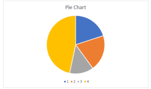
The pie chart above represents the distribution of the marital status of the study participants within the dataset. From the dataset, figures 1,2,3, and 4 represent the participants’ marital status, with 1 representing single, 2 representing married, 3 representing separated, and 4 representing widowed. Therefore, based on Figure 1, it is clear that most of the study participants from the dataset were widowed, given the largest slice of the pie is 4.
Bar Chart
Figure 2
Marital Status Bar Chart
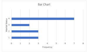
The bar chart above represents the distribution of the various marital status of the study participants. From the dataset, figures 1,2,3, and 4 represent the participants’ marital status, with 1 representing single, 2 representing married, 3 representing separated, and 4 representing widowed. Therefore, based on Figure 2 above, it is evident that most of the study participants from the dataset were widowed, given the largest bar of the bar chart is 4 widowed.
Scatterplot
Figure 3
Income vs. Age Scatterplot
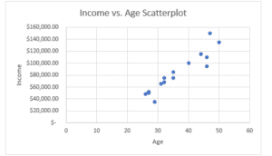
The scatterplot above represents the relationship between the age and income earned by the study participants. From Figure 3 above, one can see that as the age increases, so does the income. This means that as one gets older, their income is increased. The scatterplot also shows a positive relationship between age and income.
Histogram
Figure 4
Education levels Histogram
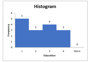
Figure 4 above represents the distribution of the various education levels of the study participants. The education levels are divided into four categories, with 1 representing Diploma, 2 representing Associate, 3 representing Bachelor, and 4 representing Masters. From the histogram, we can conclude that most of the study participants have a Diploma education level, given that the highest frequency of 5 falls within this category. We can also conclude that the education level with the least participants is Masters.
References
Costacurta, J., Duncker, L., Sheffer, B., Gillis, W., Weinreb, C., Markowitz, J., Datta, S. R., Williams, A., & Linderman, S. (2022). Distinguishing discrete and continuous behavioral variability using warped autoregressive HMMs. Advances in Neural Information Processing Systems, 35, 23838–23850. https://proceedings.neurips.cc/paper_files/paper/2022/hash/96b3aa81a9e593ca5e9b184756034a43-Abstract-Conference.html
Kaliyadan, F., & Kulkarni, V. (2019). Types of variables, descriptive statistics, and sample size. Indian Dermatology Online Journal, 10(1), 82–86. ncbi. https://doi.org/10.4103/idoj.IDOJ_468_18
Microsoft Corporation. (2018). Microsoft Excel (Version 2019) [Software]. Microsoft.
Williams, M. N. (2021). Levels of measurement and statistical analyses. Meta-Psychology, 5. https://doi.org/10.15626/mp.2019.1916
Zhang, Z., Yang, Y., & Balakrishnan, N. (2023). On conditional spacings from heterogeneous exponential random variables. Communications in Statistics – Simulation and Computation, 1–12. https://doi.org/10.1080/03610918.2023.2200914
ORDER A PLAGIARISM-FREE PAPER HERE
We’ll write everything from scratch
Question 
instructions
In this lesson’s assignment, you will complete a problem set in which you address levels of data and types of variables. Answers to the problems must be complete and written in formal narrative language. In addition, you will write a short essay related to data privacy. You will also explore the different types of graphs used to visualize data. Results from both Excel and SPSS should be copied and pasted into a Word document for submission.
Understanding Data Through Levels of Measurement and Variable Types
Explain the concept of a random variable. Explain what it means to say, “Variables must vary.” Why is the concept of variables important for learning statistics?
List and define the four levels of measurement (using examples) discussed in this lesson’s introduction and resources. In your opinion, which one or more is the most appropriate for statistical analysis? Explain.
Compare and contrast the characteristics of continuous and discrete variables. What is a common challenge of trying to calculate statistics using discrete variables?
Identify example variables from your professional and personal life at each level of measurement. Explain why you selected the level you did for each, relying on this lesson’s resources for support.
Identify at least 4 (two of each) discrete and continuous variables from your own professional or personal life and explain why you selected the category you did for each, relying on this lesson’s resources for support.