Final Course Project Worksheet and Reflection

Complete Parts A and B below.

Part A: Final Course Project Worksheet

Part A of this worksheet provides you the opportunity to synthesize your work from the entire term into a comprehensive project. Complete each section below. You will use the information from each week throughout the class (revised in line with feedback from your instructor) to paste in the appropriate material and summary. The format of this part of the worksheet is similar to what you would find as the required structure in a peer-reviewed journal.

Project Title

Impact of Education Level and Political Ideology on Attitudes Toward Healthcare Spending in the United States: Final Course Project Worksheet and Reflection.

Name

[Enter your name.]

Introduction

In the past decade, the national discussion about healthcare spending has become one of the most prominent issues in both public and policy discussions in the United States, driven by various factors that shape the opinions of the general public regarding healthcare spending. The paper examines the interactive effects of educational attainment and political ideology on the likelihood that respondents perceive national health spending as too little. Previous literature has established that both educational background and political orientation represent crucial components in the formation of preference development in healthcare policy issues (Vilhjalmsson, 2016).

Understanding these relationships takes on greater relevance in light of the current national discussion about healthcare reform and spending priorities. The intersection of education and political ideology with the attitudinal orientation on spending for healthcare provides further insight into how socio-political factors influence public policy preferences. This paper adds to the literature by considering the relative influence of education attainment and political views on general healthcare spending attitudes and offers useful lessons for policymakers and healthcare administrators in understanding public sentiments toward healthcare funding allocation.

Methodology

Research Question

What impact do education level and political ideology have on attitudes toward healthcare spending among adults in the United States?

Null and Alternate Hypothesis

Null Hypothesis

There is no significant relationship between education level, political ideology, and attitudes toward national healthcare spending.

Alternate Hypothesis

Higher education levels and more liberal political ideologies are associated with greater support for increased national healthcare spending.

Independent Variables and Levels of Measurement

Independent Variable 1: Education Level (DEGREE)

Independent Variable 2: Political Views (POLVIEWS)

Dependent Variable and Levels of Measurement

Dependent Variable: Healthcare Spending (NATHEAL)

Population and Sample

In the present analysis, three variables were selected in the attempt to explain attitudes about national healthcare spending: Education Level is DEGREE, Political Views are POLVIEWS, and Healthcare Spending is NATHEAL. An education level scale ranging from 0 (less than high school) to 4 (graduate degree) and a political views scale ranging from 1 (extremely liberal) to 7 (extremely conservative) were the independent variables that may affect attitudes about healthcare spending.

The dependent variable of healthcare spending is based on responses of 1-too little, 2-about right, or 3-too much. The study attempts to test a hypothesis that the larger the size of education and the more liberal the political ideology, the more support there is for spending on health care. In light of combining both the continuous and categorical data, a point biserial correlation is used to examine these associations (Bonett, 2019).

G*Power Output:

The G*Power output provided the following results:

• Noncentrality parameter δ: 2.9439
• Critical t: 2.0639
• Degrees of freedom (Df): 24
• Total sample size: 26
• Actual power: 0.8063

From the G* Power analysis, the recommended sample size is 26.

Results

Descriptive Statistics

Frequency Table for Independent Variable 1

Independent Variable 1 Name: Degree

Frequency Table:

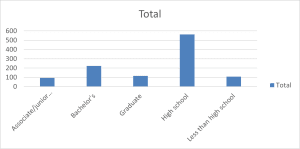
Row Labels	Count of degree
Associate/junior college	95
Bachelor’s	224
Graduate	116
High school	563
Less than high school	109
Grand Total	1107

Summary and Description:

The frequency table presents a comprehensive analysis of educational attainment among 1,107 respondents in the survey. The data reveals a significant concentration at the high school education level, with 50.9% (n=563) of respondents having completed this level of education. This majority suggests a foundational level of educational achievement within the sample population. Bachelor’s degree holders constitute the second-largest group at 20.2% (n=224), indicating a substantial proportion with higher education credentials.

Graduate degree holders represent 10.5% (n=116) of the sample, demonstrating advanced academic achievement. Those with associate/junior college degrees make up 8.6% (n=95), while 9.8% (n=109) have less than a high school education. According to Cahalan et al. (2022), this distribution generally mirrors national trends in educational attainment, though with slightly higher representation in the high school completion category than typical national averages. The relatively small percentage of respondents with less than a high school education might suggest increasing accessibility to basic education or potential sampling characteristics.

Frequency Table for Independent Variable 2

Independent Variable 2 Name: Polviews

Frequency Table:

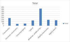
Row Labels	Count of Polviews
Conservative	186
Extremely conservative	44
Extremely liberal	54
Liberal	129
Moderate, middle of the road	417
Slightly conservative	143
Slightly liberal	134
Grand Total	1107

Summary and Description:

The frequency distribution of political views among the 1,107 respondents showcases the complex ideological landscape of the sample population. The predominant category is “Moderate, middle of the road” at 37.7% (n=417), suggesting a significant centrist orientation within the sample. Conservative viewpoints show interesting gradation, with 16.8% (n=186) identifying as Conservative, 12.9% (n=143) as Slightly conservative, and 4% (n=44) as Extremely conservative. Similarly, on the liberal spectrum, 11.7% (n=129) identify as Liberal, 12.1% (n=134) as Slightly liberal, and 4.9% (n=54) as Extremely liberal.

Wilson et al. (2020) note that this pattern of ideological distribution, with strong, moderate representation and declining numbers toward the extremes, is characteristic of contemporary political alignment patterns. The relatively small proportions at the extreme ends of the spectrum (Extremely conservative and Extremely liberal) suggest that most respondents tend to avoid identifying with more radical political positions, preferring more moderate stances.

Frequency Table for Dependent Variable

Dependent Variable Name: Natheal

Frequency Table:

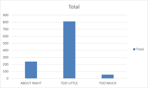
Row Labels	Count of Natheal
ABOUT RIGHT	240
TOO LITTLE	812
TOO MUCH	55
Grand Total	1107

Summary and Description:

The frequency distribution for attitudes toward healthcare spending presents a striking pattern among the 1,107 respondents, revealing strong public sentiment regarding healthcare resource allocation. An overwhelming majority of 73.4% (n=812) believe that “TOO LITTLE” is being spent on healthcare, indicating a robust public consensus for increased healthcare funding. This substantial majority suggests widespread dissatisfaction with current healthcare spending levels across the sample population. The second largest group, comprising 21.7% (n=240) of respondents, considers current spending levels “ABOUT RIGHT,” representing a smaller but significant segment satisfied with existing healthcare expenditure.

Notably, only a very small minority of 5% (n=55) believes “TOO MUCH” is being spent on healthcare. The stark imbalance in these responses, with nearly three-quarters of respondents favoring increased spending, points to a clear public mandate for healthcare funding enhancement. This distribution could reflect growing public awareness of healthcare system challenges, increasing healthcare costs, or broader concerns about healthcare accessibility and quality in the current system.

Histograms and Graphs

Histogram for Independent Variable 1

Independent Variable 1 Name: Degree

Histogram:

Summary and Description:

The histogram displays the distribution of educational attainment across five distinct categories among 1,107 respondents. The data visualization reveals a pronounced right-skewed distribution with a dominant peak at the high school education level (n=563), which towers significantly above other educational categories. Bachelor’s degree holders represent the second-highest frequency (n=224), creating a notable secondary peak in the distribution.

Graduate degree holders (n=116) and those with less than high school education (n=109) show similar frequencies, while associate/junior college degree holders represent the smallest group (n=95). The stark elevation of the high school category, combined with the gradual decline in frequency for both higher and lower educational levels, creates an asymmetrical distribution pattern.

Histogram for Independent Variable 2

Independent Variable 2 Name: Polviews

Histogram:

Summary and Description:

The histogram illustrates the distribution of political views among 1,107 respondents, revealing a distinctive bell-shaped pattern with a pronounced central peak. The data shows “Moderate, middle of the road” as the dominant category with approximately 417 respondents, creating a clear central tendency in the distribution. This peak is flanked by relatively symmetrical distributions on both the conservative and liberal sides of the spectrum.

Moving from the center, the frequencies gradually decrease toward the extremes, with “Slightly conservative” (n=143) and “Slightly liberal” (n=134) showing similar frequencies, followed by “Conservative” (n=186) and “Liberal” (n=129) maintaining comparable levels. The extremes of the political spectrum show the lowest frequencies, with “Extremely conservative” (n=44) and “Extremely liberal” (n=54) representing the smallest groups.

Histogram for Dependent Variable

Dependent Variable Name: Natheal

Histogram:

Summary and Description:

The histogram depicting attitudes toward healthcare spending among 1,107 respondents reveals a dramatically skewed distribution with a dominant preference for increased healthcare spending. The visualization shows an overwhelming majority of respondents (n=812) believing “TOO LITTLE” is being spent on healthcare, creating a pronounced peak that dwarfs the other response categories. This striking imbalance suggests a strong consensus among respondents regarding the inadequacy of current healthcare spending levels. The second category, “ABOUT RIGHT” (n=240), shows substantially lower frequency, representing just over a quarter of the peak category.

Most notably, the “TOO MUCH” category shows minimal representation (n=55), creating a sharp negative skew in the distribution. Larsen (2020) notes such strongly skewed distributions in healthcare policy preferences often indicate significant public concern about healthcare resource allocation and accessibility. The dramatic disparity between those believing too little is spent versus too much suggests a clear public mandate for increased healthcare funding, potentially reflecting broader societal concerns about healthcare affordability and access. The minimal support for reduced spending, combined with the modest satisfaction with current levels, creates a distribution pattern that strongly favors policy initiatives supporting expanded healthcare investment.

Independent Variable 1

Independent Variable 1 Name: degree

Descriptive Statistics Table:

Degree Recoded
Mean	1.706414
Standard Error	0.036055
Median	1
Mode	1
Standard Deviation	1.199602
Sample Variance	1.439046
Kurtosis	-0.85605
Skewness	0.601744
Range	4
Minimum	0
Maximum	4
Sum	1889
Count	1107

Summary and Description:

The Education Level variable (degree), coded from 0 to 4, represents the respondents’ highest degree attained, from less than high school to a graduate degree. The mean degree level was 1.71, indicating a central tendency toward high school-level education, with the median and mode both at 1. This central clustering reflects a predominant high school-level education among respondents, with a limited representation of graduate degree holders. With a standard deviation of 1.20, the data shows moderate variability, capturing diverse educational attainment but with a skew toward lower education levels, possibly reflective of broader population trends.

Independent Variable 2

Independent Variable 2 Name: Polviews

Descriptive Statistics Table:

Polviews Recoded
Mean	4.084011
Standard Error	0.044378
Median	4
Mode	4
Standard Deviation	1.476515
Sample Variance	2.180097
Kurtosis	-0.46583
Skewness	-0.11632
Range	6
Minimum	1
Maximum	7
Sum	4521
Count	1107

Summary and Description:

Political Views (polviews) range from 1 (extremely liberal) to 7 (extremely conservative), average at a mean score of 4.08. This central score, along with a median and mode of 4, indicates that most respondents identify as moderate. The standard deviation of 1.48 reflects a fairly balanced spread across the spectrum from liberal to conservative views, indicating ideological diversity in the sample.

The slight negative skew suggests a mild leaning toward more liberal stances, though the distribution remains relatively balanced around the midpoint. This variable provides a nuanced snapshot of political ideology within the surveyed group.

Dependent Variable

Dependent Variable Name: Natheal

Descriptive Statistics Table:

Natheal Recoded
Mean	1.31617
Standard Error	0.016892
Median	1
Mode	1
Standard Deviation	0.562014
Sample Variance	0.315859
Kurtosis	1.572727
Skewness	1.600474
Range	2
Minimum	1
Maximum	3
Sum	1457
Count	1107

 Summary and Description:

Healthcare Spending, coded from 1 (too little) to 3 (too much), shows a mean of 1.32, suggesting a predominant perception that current spending on healthcare is insufficient. With the median and mode both at 1, the data indicates a strong consensus among respondents in favor of increased spending. The standard deviation of 0.56 points to low variability, highlighting general agreement on this issue. Skewness and kurtosis values further support this clustering around “too little” spending, providing valuable insights into public opinion on national healthcare investment.

Measures of Variability

Independent Variable 1

Justification:

The ordinal scale “Education Level” is measured on a scale ranging from 0 (Less than high school) through 4 (Graduate degree). Since some categories are not equidistant, the IQR is the appropriate measure of variability for an ordinal variable with no equal intervals between categories (Gravetter & Wallnau, 2017). The IQR is especially well-fit for ordinal data because it orients itself to the middle 50% of responses and does not support the assumption of equal distances, an assumption which would be inappropriate when educational levels can vary considerably in both effort and length.

Most importantly, the IQR gives a dispersion measure that resists outliers or extremes, hence providing representative measures of central tendencies (Field, 2018). The use of IQR avoids overstating variability due to unequal intervals between education levels while focusing on the spread around the median, which becomes key in drawing patterns within educational attainment.

Level of Measurement:

Ordinal

Measure of Variation Table:

Statistic	Value
Minimum	0
First Quartile (Q1)	1
Median	1
Third Quartile (Q3)	3
Interquartile Range (IQR)	2

Summary of Table Results:

The interquartile range for Education Level from the above table is 2, indicating a medium spread between respondents. This range indicates that the middle 50% of responses are spread between the high school level and the bachelor’s degree level. Clustering around these levels forms a pattern that the majority of respondents either hold a high school diploma or undergraduate degree, which composes a foundational trend for the level of education in this sample. In support, Gravetter and Wallnau (2017) cite that IQR stands useful in ordinal data to reflect actual trends without distorting from extreme values.

Consequently, with this response population having a central concentration, a classic educational distribution is somewhat typical of greater trends in comparable populations. In this way, the distribution would suggest that there is limited sample variation at both the lowest and highest levels of education, which can be a specific factor in determining perceptions about various sociocultural phenomena of interest, including political views and attitudes toward national policies.

Independent Variable 2

Justification:

“Political Views” is an ordinal variable as well. Responses range from 1 (Extremely liberal) to 7 (Extremely conservative). Similar to Education Level, there are no equal intervals between each category, so IQR would be the best measure of variability. It better represents the middle 50% of the responses, unlike when the spacing between categories is unequal.

The IQR gives an accurate reflection on ideological diversity in the sample (Field, 2018). Here, IQR is selected because it can summarize the spread of the middle part of the data that measures respecting the natural properties of ordinal data measurement are created this way (Trochim et al., 2016). Since some data on political views might be skewed, IQR will allow observation of variation without much affection by extreme liberal or conservative answers and thus hold the integrity of the analysis in trying to obtain a balanced overview of politics.

Level of Measurement:

Ordinal

Measure of Variation Table:

Statistic	Value
Minimum	1
First Quartile (Q1)	3
Median	4
Third Quartile (Q3)	5

Summary of Table Results:

The interquartile range for the variable Political Views is 2, indicating that most respondents identify closer to the middle of the ideological spectrum, with scores clustering between “Slightly liberal” and “Slightly conservative.” This finding is supported by the median score of 4, which reflects centrist or moderate orientation. The distribution of political views is bell-shaped, peaking in moderate viewpoints that reflect the tendency of respondents to shy away from extreme positions.

According to Gravetter and Wallnau (2017), by focusing on the middle 50%, the IQR will give insight into the core spread of responses by providing a look at variability that respects symmetry in the distribution around the median. This moderate spread across middle categories gives grounds for diversity, yet epidemiological balance in ideological perspectives within the sample, with subconscious emergence of a single common element of respondents, such as average political leanings.

Dependent Variable

Justification:

The “Healthcare Spending” variable is ordinal because the values are coded from 1 (Too little) to 3 (Too much). As with the other variables, IQR is chosen because the nature of the variable is ordinal. IQR is preferred for an ordinal variable because it allows for a focus on the variation in the central responses, and it does not impose any assumptions about the distribution of distances between “Too little,” “About right,” and “Too much” variables.

IQR serves well to communicate the public’s opinion on spending about healthcare and, more specifically, whether there is a significant dispersion around the preferred response, “Too little,” without giving too much weight to the outliers. In this manner, it depicts a real sense of variation by focusing on responses that reflect the opinion of the majority without being skewed.

Level of Measurement:

Ordinal

Measure of Variation Table:

Statistic	Value
Minimum	1
First Quartile (Q1)	1
Median	1
Third Quartile (Q3)	2
Interquartile Range (IQR)	1

Summary of Table Results:

The Healthcare Spending-Interquartile range is 1. This would suggest there is strong clustering around the belief that current spending is “Too little.” The median is 1, and the mode is also 1; this suggests uniform agreement among respondents with the belief that more money needs to be spent on healthcare, supporting low variability of opinion. Field (2018) adds that such a small spread in an ordinal variable may mean a similar view among the people, which reiterates that in issues such as healthcare funding, interpretation should be stretched to the level of public opinion.

The IQR does not spread out much; this means most of these responses fall in the “More Spending” category, hence critical in bringing out societal values and policy preferences. This is in tandem with the social trend that citizens would wish to have more investment in health, as described by Trochim et al. (2016), which might have a strong influence on public policy and the issue of politics.

Measures of Association and Tests of Significance

The statistical test chosen for the variables was regression. Regression analysis is one of the appropriate statistical methods to be used if the relationship between one or more independent variables and a dependent variable is to be measured (Sarstedt & Mooi, 2018). In this case, it is the healthcare spending attitude as represented by the variable ‘NATHEAL’, which is ordinal in nature. However, for this analysis, the variable is assumed to be continuous to allow for regression analysis.

The independent variables are the highest degree earned, which is a measure of education level or DEGREE, and political views or POLVIEWS put on a liberal-to-conservative scale. Regression is preferred to analyze how these predictors jointly affect attitudes toward healthcare spending. It is appropriate since the method has indicated the strength and statistical significance of these relationships that might be used to understand those factors that shape opinions on healthcare spending.

The regression analysis was run using Excel, and the output below was obtained.

SUMMARY OUTPUT
Regression Statistics
Multiple R	0.168056
R Square	0.028243
Adjusted R Square	0.026482
Standard Error	0.554522
Observations	1107
ANOVA
	df	SS	MS	F	Significance F
Regression	2	9.866365	4.933182	16.04314	1.35E-07
Residual	1104	339.4742	0.307495
Total	1106	349.3406
	Coefficients	Standard Error	t Stat	P-value	Lower 95%	Upper 95%	Lower 95.0%	Upper 95.0%
Intercept	1.022719	0.056997	17.94334	2.26E-63	0.910884	1.134554	0.910884	1.134554
Degree	0.019293	0.013987	1.379341	0.168069	-0.00815	0.046737	-0.00815	0.046737
Polviews	0.063792	0.011364	5.613614	2.51E-08	0.041495	0.08609	0.041495	0.08609

The regression analysis gave an important insight into the relationship between the level of education, political views, and attitude toward healthcare expenditure. The F-statistic with its value of 16.043 and the p-value with a value of 1.35E-07 gave support that the combined effect of independent variables causes a significant difference in the dependent variable; however, seeing the value of R², which was 0.028, the explanatory power of the model would be quite low.

This suggests that although the relationship of the predictors to the outcome is statistically significant, the model accounts for only 2.82% of the variance in attitudes toward national healthcare spending. More literally, though the predictors contribute significantly to understanding healthcare spending attitudes, other factors not included in the model are likely to play a larger role.

Further contextualization is reinforced by analyzing each of the independent variables. The education level variable, DEGREE, has an estimated coefficient of 0.019; this is indicative of a weak positive slope between greater educational attainment and the likelihood of increased support for national healthcare spending. However, the p-value for this variable, at 0.168, exceeds the conventional threshold for statistical significance at p < 0.05.

That might indicate some evidence that higher education can lead to more significant support for healthcare spending, but the evidence does not appear strong enough to determine with any confidence that this relationship is statistically significant in this data set. Therefore, education level might not be a reliable predictor of healthcare spending attitudes in this particular setting.

On the other hand, POLVIEWS are significantly related to attitudes toward spending on healthcare. The coefficient of political views is 0.064, indicating that every step toward conservative political views decreased the attitude of support for additional spending on healthcare. This is highly significant, as its resultant p-value stands at 2.51E-08, which is far below the 0.05 level.

This is in agreement with the literature, which denotes that political ideology strongly predicts general public attitudes toward priorities in government spending and healthcare (Vilhjalmsson, 2016). More conservative subjects are for limited government intervention, and thus, they would predictably support increases in national health spending less than their opponents.

These results highlight how political ideology explains much of the variance in public attitudes about spending on healthcare, while the role of education is less influential based on this dataset. The overall low R² would also support that while the political view is significant, it is but one factor in a myriad that affects this attitude. Such factors as income, demographics, and personal experiences with healthcare might be considered as other predictors in constructing a complete model of attitudes toward healthcare spending in future studies. This would provide greater clarity on the complex interconnection of factors driving public opinion in this domain.

Discussion

The analysis shows several meaningful results on how educational level and political ideology might be related to general attitudes toward healthcare spending in a sample of U.S. adults. The results are complex and show nuances in how these variables combine to present public views about healthcare spending.

The most striking finding is the general support throughout the sample for more healthcare spending: 73.4% of respondents characterized present spending as “too little.” This strong consensus supports the belief that the perception of inadequate healthcare funding cuts across education and political lines. Factors influencing these attitudes show various degrees of impact.

Political ideology is a stronger predictor of healthcare spending attitude since the relationship has become statistically significant: p = 2.51E-08. The coefficient of 0.064 for political views is positive, which indicates that more conservative ideological positions are associated with decreased support for additional healthcare spending. This makes sense because traditional conservative ideology would favor limited government intervention and reduced public spending.

Surprisingly, education level relates to healthcare spending attitudes in a much weaker way than one would have expected. While there is a slight positive correlation, with higher education levels being associated with support for more healthcare spending, the coefficient = 0.019, the relationship did not reach statistical significance, p = 0.168. This may indicate that formal education has a less decisive role in shaping attitudes toward healthcare spending than previously assumed.

The overall model is statistically significant at F = 16.043, p = 1.35E-07, but it explains only a small portion of the variance in healthcare spending attitudes, with R² = 0.028. The relatively low explanatory power of this model suggests that other factors not taken into consideration by the model are likely to play substantial roles in determining attitudes toward healthcare spending. Such factors might include personal experiences with healthcare, income levels, age, or direct exposure to healthcare systems.

Frequency distribution across variables shows interesting patterns. In educational attainment, there is a concentration at the high school level, 50.9%, while in political views, there is a normal distribution with centrality on moderate positions, 37.7%. This is indicative that the sample generally represents typical demographic patterns and thus gives credence to the findings.

Conclusion

This study helps gain insight into what may account for public attitudes in the United States regarding healthcare spending. Whereas political ideology certainly emerges as an important predictor of healthcare spending attitudes, the relationship between spending preferences and educational attainment seems to be more nuanced than initially hypothesized. The findings have major implications for policymakers and health administrators when understanding public sentiment toward healthcare funding allocation.

Where future studies might develop this more comprehensively by incorporating variables of income levels, personal healthcare experiences, and demographic factors into a proposed model of healthcare spending attitude. Longitudinal research can further indicate how the trends change with time, possibly in relation to any modification or framing of policies. Overall, the uniform, great citizen demand for increased healthcare expenditure regardless of educational level seems to need discussions at broader public policy talks about healthcare funding priorities and resources.

The limitations of this present study, in particular its overall low R-squared, suggest that, although political ideology and education level make significant contributions to an explanation of attitudes toward spending on healthcare, they form a part of a much more complex matrix of influences upon the public view of this issue. Further studies may usefully employ qualitative research to enhance the depth of insight into the underlying reasoning that these attitudes and preferences display.

References

Bonett, D. G. (2019). Point‐biserial correlation: Interval estimation, hypothesis testing, meta‐analysis, and sample size determination. British Journal of Mathematical and Statistical Psychology. https://doi.org/10.1111/bmsp.12189

Cahalan, M. W., Addison, M., Brunt, N., Patel, P. R., Vaughan, T., Genao, A., & Perna, L. W. (2022). Indicators of higher education equity in the United States: 2022 historical trend report. In ERIC. Pell Institute for the Study of Opportunity in Higher Education. https://eric.ed.gov/?id=ED620557

Field, A. (2018). Discovering statistics using IBM SPSS statistics (5th ed.). Sage Publications.

Gravetter, F. J., & Wallnau, L. B. (2017). Statistics for the behavioral sciences (10th ed.). Cengage Learning.

Larsen, E. G. (2020). Personal politics? Healthcare policies, personal experiences and government attitudes. Journal of European Social Policy, 095892872090431. https://doi.org/10.1177/0958928720904319

Sarstedt, M., & Mooi, E. (2018). Regression analysis. In Springer texts in business and economics (pp. 209–256). https://doi.org/10.1007/978-3-662-56707-4_7

Trochim, W. M. K., Donnelly, J. P., & Arora, K. (2016). Research methods: The essential knowledge base. Cengage Learning

Vilhjalmsson, R. (2016). Public views on the role of government in funding and delivering health services. Scandinavian Journal of Public Health, 44(5), 446–454. https://doi.org/10.1177/1403494816631872

Wilson, A. E., Parker, V. A., & Feinberg, M. (2020). Polarization in the contemporary political and media landscape. Current Opinion in Behavioral Sciences, 34(2352-1546), 223–228. https://doi.org/10.1016/j.cobeha.2020.07.005

Part B: Reflection

How does the type of data drive statistical tests used?

Fundamentally, the nature of the data collected within a research study dictates the type of statistical test that can be applied. Data are categorized into four levels of measurement: nominal, ordinal, interval, and ratio. Each level prescribes certain statistical procedures that will yield meaningful and valid analysis. For instance, Gravetter and Wallnau (2017) indicate that the appropriate selection of a test that fits the measurement level of the data provides a basis for valid interpretations.

Nominal data represents categories without value, like gender or political affiliation, necessitates the use of non-parametric tests, often in the form of chi-square tests of association or frequency. Ordinal data represents rank or order but without equal intervals, such as through the utilization of Likert scales, and lends itself to median comparisons or non-parametric tests, such as the Mann-Whitney U test.

Interval and ratio data are jointly called continuous data because they both have numerical values that can support more elaborate statistical methods. Examples of this would be t-tests, ANOVA, or regression analyses, which presuppose an interval level of measurement or higher. An example of such can be seen in the work carried out in this class that examined the association of educational attainment and political ideology with views on healthcare spending (both ordinal) that relied on appropriate measures of central tendency and regression models in response to the data types being tested.

Field (2018) argues that the basis of regression models involves understanding data properties, hence the need to develop tests that match data types. Understanding the type of data enables one to apply statistical tests that are consistent with its assumptions to ensure that one will not make incorrect conclusions. Such a relation of data properties with test applicability was emphasized during the week, especially when discussions related to variable measurement and hypothesis testing were made.

Why is it important to understand the types of data, research question, hypotheses, etc., prior to determining which statistical test is most appropriate?

The selection of proper statistical tests depends on a good understanding of the nature of the data, research questions, and hypotheses. The research question will define the relationship or comparison of interest, while the hypothesis will provide a framework for testing those relationships. Without clarity on those foundational elements, it is easy to apply inappropriate statistical methods, which lead to invalid results. Trochim et al. (2016) note that well-defined hypotheses guarantee appropriate test selection for the research questions being put forward.

For example, this project examined how educational attainment and political ideology impact attitudes on healthcare spending. Identifying the dependent variable as an attitude toward healthcare spending and the independent variables as education level and political ideology directed the study to regression analysis. The knowledge that each of these is an ordinal-level variable prevented incorrect uses of parametric tests, which assume interval data.

Additionally, a good judgment about data characteristics, particularly normality, dispersion, and scale, enables one to improve test selection. For example, assumptions of a normal distribution and homogeneity of variance make the use of t-test parametric tests instead of non-parametric tests. Identifying these things beforehand avoids misinterpretation of the results.

For instance, the G*Power analysis done within this project brought out sample size requirements alone, showing how planning influences statistical power and validity. By integrating these principles from the weekly lessons, such as measurement of variables, formulation of hypotheses, and selection of tests, as indicated by Sarstedt and Mooi (2018), I acquired a step-by-step manner of conducting quantitative analysis. This foundational knowledge supports the integrity of research outcomes.

Reflect on your experience in this class. What information did you find most useful? How will you apply this information moving forward in your academic or professional life?

This course has provided a broad overview of the concepts of statistics and how they might be applied to social research. The procedures for choosing appropriate statistical tests and interpreting the results were included. Since it was developed from the beginning with concepts of data types and variable measurement to more advanced topics like regression analysis, this class cohesively presented concepts interconnected in the process of decision-making in statistics. Trochim et al. (2016) provided foundational insight into the role of structured analysis frameworks within research.

I found the application of G*Power in determining sample size and statistical power particularly enlightening. The tool showed the importance of planning in research design by ensuring adequate power is present to detect significant effects. Furthermore, the emphasis on how to interpret descriptive and inferential statistics, especially in understanding regression coefficients and p-values, further developed my critical thinking in evaluating research findings.

Moving forward, I will use these skills in academic and professional pursuits. In my academics, the knowledge serves as a framework for carrying out robust quantitative research, from formulating a research question to the execution and interpretation of analyses. Professionally, this would become helpful, particularly in those professional roles that have to solve problems with some basis in data.

This course has equipped me with several analytical tools for approaching multi-faceted questions in a coherent manner, with rigor and accuracy in research and practice. I will take these foundational pieces and build further to refine my statistical acumen, with which to meaningfully contribute to my field.

References

Field, A. (2018). Discovering statistics using IBM SPSS statistics (5th ed.). Sage Publications.

Gravetter, F. J., & Wallnau, L. B. (2017). Statistics for the behavioral sciences (10th ed.). Cengage Learning.

Sarstedt, M., & Mooi, E. (2018). Regression analysis. In Springer texts in Business and Economics (pp. 209–256). https://doi.org/10.1007/978-3-662-56707-4_7

Trochim, W. M. K., Donnelly, J. P., & Arora, K. (2016). Research methods: The essential knowledge base. Cengage Learning.

ORDER A PLAGIARISM-FREE PAPER HERE

We’ll write everything from scratch

---

RES 710 Week 8 Assignment