Hypothesis Testing – Blood Pressure
Hypotheses formulated in the previous module
- Null Hypothesis (H0): The range for the recorded blood pressure values indicates that the individual is not healthy/at risk.
- Alternative Hypothesis (H1): The range for the recorded blood pressure values indicates the individual is healthy.
- Appropriate Test Statistics to evaluate the evidence against the null hypothesis
The test statistic that appropriately provides evidence against the null hypothesis is a t-test. The t-test compares the means for the systolic and diastolic values between the hypothesized data and the normal systolic and diastolic values (Norman & Streiner, 2014). Therefore, the analysis will take alpha at 0.05 to test whether the values are less than or equal to 120/80mmHg
Our assignment writing services will allow you to attend to more important tasks as our experts handle your task.
Why the t-test was chosen
A paired t-test will be suitable since the systolic and diastolic data values are obtained from a single sample population. Further, the t-test is suitable since the sample size is less than 30 and the standard deviation can be obtained, making it fit the test criteria (Trochim, 2006). To determine whether there is a significant difference between the normal blood pressure recording and the hypothesized recordings in the data table, it can be computed manually or using statistical analysis software (StatisticsHowTo, 2020).
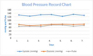
Summary Graph for the Data
| Day | Time | Systolic (mmHg) | Diastolic (mmHg) | Pulse |
| 1. | 8:50:00 AM | 131 | 77 | 66 |
| 2. | 9:06:00 AM | 124 | 70 | 67 |
| 3. | 9:48:00 AM | 132 | 73 | 65 |
| 4. | 8:40:00 AM | 133 | 78 | 73 |
| 5. | 10:00:00 AM | 123 | 79 | 73 |
| 6. | 9:05:00 AM | 134 | 77 | 67 |
| 7. | 11:15:00 AM | 129 | 79 | 71 |
Figure 1: Summary Graph for Blood Pressure Data Recordings
| t-Test: Paired Two Sample for Means | ||
| Systolic (mmHg) | Diastolic (mmHg) | |
| Mean | 129.4285714 | 76.14285714 |
| Variance | 18.95238095 | 11.47619048 |
| Observations | 7 | 7 |
| Pearson Correlation | 0.198575223 | |
| Hypothesized Mean Difference | 0 | |
| Df | 6 | |
| t Stat | 28.44098337 | |
| P(T<=t) one-tail | 6.25432E-08 | |
| t Critical one-tail | 1.943180281 | |
| P(T<=t) two-tail | 1.25086E-07 | |
| t Critical two-tail | 2.446911851 |
Table 1: Excel Analysis Output for Blood Pressure Observations
From the analysis, the p-values for both one-tailed and two-tailed are less than the critical values; thus, we accept the null hypothesis that the individual is not healthy. Mean systolic blood pressure is above the expected normal (120mmHg), but the diastolic pressure is within range. The individual is at risk of hypertension if systolic values go beyond the current mean.
Sample size, error, and accuracy of the analysis
The sample size for the above observations is seven. The sample has a higher possibility of measurement error due to the small sample size. Field (2008) explains that the larger the sample size, the smaller the error. It is justified to conclude that the sample is too small for accurate deductions about the individual’s risk of hypertension.
References
Field A. (2018) Discovering Statistics Using IBM SPSS Statistics, Sage Publishers, California.
Norman, G. R., & Streiner, D. L. (2014). Section the second: Analysis of variance. Chapter 7: Comparing two groups. In Biostatistics: The bare essentials [4th Ed.]. Shelton, ISBN-13: 978-1-60795-279-4
StatisticsHowTo (2020). “T Test (Student’s T-Test): Definition and Examples” Retrieved from: https://www.statisticshowto.com/probability-and-statistics/t-test/
Trochim, W. (2006). The t-test. Research Methods Knowledge Base. Retrieved from: http://www.socialresearchmethods.net/kb/stat_t.php
ORDER A PLAGIARISM-FREE PAPER HERE
We’ll write everything from scratch
Question

Hypothesis Testing – Blood Pressure
Having developed the null and alternative hypotheses in the previous module, write a (2-3 pages) paper in which you:
Identify a test statistic to help you assess the evidence against the null hypothesis you developed in the previous module.
Explain why you have chosen the specific test statistic. Include a description of the test statistic in your discussion.
Summarize your findings by creating a summary graph in which you display your data.
Discuss the total number of measurements (sample size), the possibility for measurement error, and whether it is large enough to paint an accurate picture.


