Housing Price Prediction Model for D. M. Pan National Real Estate Company

Housing Price Prediction Model for D. M. Pan National Real Estate Company

Introduction

1. The current report aims at employing statistical analysis techniques for problem-solving. Particularly, the analysis involves a regression analysis to develop a model that predicts housing prices for homes sold in 2019 for D. M. Pan National Real Estate Company. The information obtained will help real-estate agents predict the median prices of the houses subject to the area in square feet.
2. The study will answer the question as to whether there exists a relationship between the house price listing and the area in square feet. This will determine if the company can use the model for price prediction.
3. The regression model is appropriate for the analysis since it shows the relationship between the variables as well as the direction of the relationship in a regression model and a scatter plot. When using a regression line, the scatter plot can either produce a straight line with an upward or a downward trend or a distribution that does not show any linear relationship.
4. The response variable is the variable that is affected by a change in the variables that predict the outcome, while the predictor variables are the variables that determine the outcome of the response variables. The variable that poses an effect on the other variable is taken as the predictor variable.

Data Collection

1. A random sample is selected from the data provided in the Excel sheet with house footage values and corresponding prices by selecting the first 50 data cells.
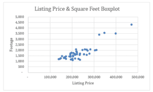
2. The square footage affects the median housing prices, thus taken as the predictor and response variables, respectively.
3. Scatter Plot for the Variables

Data Analysis

Listing Price		Square Feet
Mean	229130	Mean	1758.5
Standard Error	8912.724795	Standard Error	92.1583121
Median	216200	Median	1630
Mode	254500	Mode	2087
Standard Deviation	63022.48141	Standard Deviation	651.657674
Sample Variance	3971833163	Sample Variance	424657.724

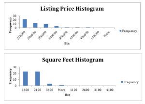
Interpret the graphs and statistics: For both variables, the mean value is larger than the median value. This shows that the values are concentrated at the center, and the shape of the distribution graphs is likely to be peaked at the center. The standard deviation for the listing is higher than the standard deviation for the square footage. Since the mean for the data is larger than the median listing price, it implies that the curves are positively skewed.

The national mean listing price is 342,365. The mean listing for the sample is smaller (229,130) than the national mean listing prices. However, for both the sample and national data, the mean listing price and the mean square footage is larger than the median listing price. This shows that the sample is fully representative of the population (Turner, 2020). The distribution curves for both the sample data and the national data are likely to be identical.

The Regression Model

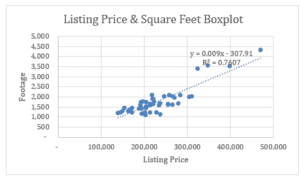
From the graph above, a regression model can be developed out of the data. The model is obtained as y= 0.009x – 307.91. Although the scatter plot may not be very accurate, it can explain 76% of the change in the variables.

Discuss associations: From the scatter plot and the trend line, there is a positive association between the house footage and the listing prices. This can be derived from the upward trend between the two variables. Removing the outliers leads to a better model.

Find r: From the regression output, the r value is 0.87. This shows a positive correlation between the two variables. The line of best fit in the scatter plot also implies a positive correlation (Salkind, 2015). The R-square value in the regression output is equal to the value in the regression graph. The regression output reflects what was obtained from the scatterplot output.

SUMMARY OUTPUT
Regression Statistics
Multiple R	0.872188
R Square	0.760713
Adjusted R Square	0.755728
Standard Error	31148.18
Observations	50

The Line of Best Fit

ANOVA
	df	SS	MS	F	Significance F
Regression	1	1.48E+11	1.4805E+11	152.5956858	1.62116E-16
Residual	48	4.66E+10	970209425.1
Total	49	1.95E+11
	Coefficients	Standard Error	t Stat	P-value	Lower 95%	Upper 95%	Lower 95.0%	Upper 95.0%
Intercept	80800.1	12790.13	6.317377178	8.19583E-08	55083.81528	106516.394	55083.82	106516.4
square feet	84.35024	6.828341	12.35296263	1.62116E-16	70.62093972	98.0795386	70.62094	98.07954

Regression equation: y= 0.009x – 307.91.

Interpret regression equation: The slope of the line is a positive gradient, which indicates a positive association between the two variables. The regression equation from the regression output is y=84.35x + 80800.1, which gives the line of best fit. The equation further indicates a positive correlation between the variables. The intercept is 80800.1. The gradient of the slope is 84.35.

Strength of the equation: The strength of the regression equation is shown by the value R-squared, which is 0.76 (76%). This implies that the regression equation explains 76% of the change in the outcome variable with a unit change in the explanatory variable. The p-value of the model is very small (p<.05, 1.62116E-16); thus, the model significantly predicts the change in the variables as well as the association.

Use the regression equation to make predictions: The regression equation can be used to make predictions about the price of houses given particular square footage. For instance, a sample prediction using the model can be obtained as;

Taking footage as 100 square feet

y=84.35x + 80800.1

= 84.35(100) + 80800.1 = 89235. Therefore, for a house that measures 100 square feet, the company can quote it as $89235. However, the management will refer to the price listing catalog for accuracy since the model predicts 76% of the price change corresponding to the floor area.

Conclusions

The analysis can be crucial for the company’s operations. It can be used to predict the prices of a house based on the house measurements in square footage. Generally, the model indicates that there is a positive association between the square footage and the house pricing. This implies that an increase in the area will indicate an increase in the price of the house. Following the output of the analysis, the analysis meets the researcher’s expectations since, logically, keeping other factors constant, the larger the size of a room, the higher the price listing. However, the model had outliers that reduced its accuracy. This could be due to the many different states from where the data is collected. Removing the outliers could yield a more accurate model. Thus, a change that could lead to a different output and results could be enhancing the homogeneity of the data points (Salkind, 2015). An interesting follow-up question for the current study could be whether location could be a significant predictor of the pricing trends in the states. Perhaps the variable could be included in the future analysis.

References

Salkind, N. (2015). Excel Statistics: A Quick Guide. Third Edition. SAGE Publications.

Turner, D. P. (2020). Sampling Methods in Research Design. Headache: The Journal of Head and Face Pain, 60(1), 8–12.

ORDER A PLAGIARISM-FREE PAPER HERE

We’ll write everything from scratch

---

In this project, you will demonstrate your mastery of the following competencies:

• Apply statistical techniques to address research problems
• Perform regression analysis to address an authentic problem

Overview

The purpose of this project is to have you complete all of the steps of a real-world linear regression research project, starting with developing a research question, then completing a comprehensive statistical analysis, and ending with summarizing your research conclusions.

Scenario

You have been hired by the D. M. Pan National Real Estate Company to develop a model to predict housing prices for homes sold in 2019. The CEO of D. M. Pan wants to use this information to help their real estate agents better determine the use of square footage as a benchmark for listing prices on homes. Your task is to provide a report predicting the housing prices based on square footage. To complete this task, use the provided real estate data set for all U.S. home sales as well as national descriptive statistics and graphs provided.

Directions

Using the Project One Template located in the What to Submit section, generate a report including your tables and graphs to determine if the square footage of a house is a good indicator of what the listing price should be. Reference the National Statistics and Graphs document for national comparisons and the Real Estate Data spreadsheet (both found in the Supporting Materials section) for your statistical analysis.

Note: Present your data in a clearly labelled table and using clearly labelled graphs.

Specifically, include the following in your report:

Introduction

1. Describe the report: Give a brief description of the purpose of your report.
   1. Define the question your report is trying to answer.
   2. Explain when using linear regression is most appropriate.
      1. When using linear regression, what would you expect the scatterplot to look like?
   3. Explain the difference between response and predictor variables in a linear regression to justify the selection of variables.

Data Collection

1. Sampling the data: Select a random sample of 50 houses.
   1. Identify your response and predictor variables.
2. Scatterplot: Create a scatterplot of your response and predictor variables to ensure they are appropriate for developing a linear model.

Data Analysis

1. Histogram: For your two variables, create histograms.
2. Summary statistics: For your two variables, create a table to show the mean, median, and standard deviation.
3. Interpret the graphs and statistics:
   1. Based on your graphs and sample statistics, interpret the centre, spread, shape, and any unusual characteristic (outliers, gaps, etc.) for the two variables.
   2. Compare and contrast the shape, centre, spread, and any unusual characteristic of your sample of house sales with the national population. Is your sample representative of national housing market sales?

Develop Your Regression Model

1. Scatterplot: Provide a graph of the scatterplot of the data with a line of best fit.
   1. Explain if a regression model is appropriate to develop based on your scatterplot.
2. Discuss associations: Based on the scatterplot, discuss the association (direction, strength, form) in the context of your model.
   1. Identify any possible outliers or influential points and discuss their effect on the correlation.
   2. Discuss keeping or removing outlier data points and what impact your decision would have on your model.
3. Find r: Find the correlation coefficient (r).
   1. Explain how the value you calculated supports what you noticed in your scatterplot.

Determine the Line of Best Fit. Clearly define your variables. Find and interpret the regression equation. Assess the strength of the model.

1. Regression equation: Write the regression equation (i.e., line of best fit) and clearly define your variables.
2. Interpret regression equation: Interpret the slope and intercept in context.
3. Strength of the equation: Provide and interpret R-squared.
   1. Determine the strength of the linear regression equation you developed.
4. Use the regression equation to make predictions: Use your regression equation to predict how much you should list your home for based on the square footage of your home.

Conclusions

1. Summarize findings: In one paragraph, summarize your findings in clear and concise plain language for the CEO to understand. Summarize your results.
   1. Did you see the results you expected, or was anything different from your expectations or experiences?
      1. What changes could support different results or help to solve a different problem?
      2. Provide at least one question that would be interesting for follow-up research.