FINAL LAB PRACTICAL–General Chemistry II Lab

FINAL LAB PRACTICAL–General Chemistry II Lab

Do you need help with your assignment ? Hire our assignment writing services in case your assignment is devastating you.

Part I: Equilibrium Constant Determination:

The equilibrium for the formation of FeSCN²⁺ has been achieved by combining 0.002 M solutions of Fe(NO₃)₃ and NaSCN.

Reaction studied:      Fe³⁺  +  SCN^1-  <=>  FeSCN²⁺, K_f = [FeSCN²⁺]/[Fe³⁺][ SCN^1-]

Based on Beer’s Law concept, we achieved a linear plot by various dilutions of reactants (these data are not given). The linear equation is shown below.

A  = 2622.52 x [FeSCN²⁺] -2.691E-4           R =  0.99965

Remember to use the formula C_iV_i = C_fV_f to determine the initial concentrations right before they react. (Note: V_f is 6.00 mL every time.)

Table 1: Initial concentration of Fe³⁺ and SCN^– solutions.                           (10 points)

Soln #	Volume of 2.00E-3 M Fe3+ (mL)	Volume of 2.00E-3 M SCN1- (mL)	Volume of water (mL)	Total Volume (mL)	[Fe3+]o M	[SCN1-]o M
Blank	3.00	0.00	3.00	6.00	1.00E-3	0
1B	1.00	3.00	2.00	6.00	3.33E-4	1.00E-3
2B	2.00	3.00	1.00	6.00	6.67E-4	1.00E-3
3B	3.00	3.00	0.00	6.00	1.00E-3	1.00E-3
4B	3.00	2.00	1.00	6.00	1.00E-3	6.67E-4
5B	3.00	1.00	2.00	6.00	1.00E-3	3.33E-4

Use Beer’s Law to determine the concentration from the absorbance provided and use ICE charts to determine the equilibrium concentrations and the K_f.

(15 points)

Soln #	Absorbance measured	[FeSCN2+]eq M	[Fe3+]eq M	[SCN1-]eq M	Kf
Blank	—	—	—	—	—
1B	0.105	0.0000399	0.0002901	0.0009601	14.33
2B	.225	0.0000857	0.0005813	0.0009143	161.25
3B	.345	0.000131	0.000869	0.000869	173.47
4B	.451	0.000172	0.000828	0.000495	419.63
5B	.564	0.000215	0.000785	0.000118	2321.06

Calculate the average K_f and its standard deviation and perform the 4D test, if necessary, i.e., based on the discarding of n unwanted value.             (5 points)

STANDARD DEVIATION

Mean = 14.33+161.25+173.47+419.63+2321.06 =3089.74/5 =617.95

x	x-mean	(x-mean)2
14.33	-603.62	364357.1044
161.25	-456	207936
173.47	-444.48	197562.47
419.63	-198.32	39330.8224
2321.06	1703.11	2900583.672
Sum=3089.74	0	3709770.069

 Variance = 3709770.069/ 5-1 = 741954.0138

 Standard deviation =

= 861.4

(a) Show calculations for the initial diluted concentrations of Fe³⁺ and SCN^– 

(5 points)

[Fe3+]o M	[SCN1-]o M
1B = CiVi = CfVf                                                                                                                             2.00E-3 M X 1.00 = 6.00 X Cf                                   Cf   = 3.333 E-4	1B = CiVi = CfVf                                                                                                                              2.00E-3 M X 3.00 = 6.00 X Cf                                   Cf   = 1.00 E-3
2B = CiVi = CfVf                                                                                                                             2.00E-3 M X 2.00 = 6.00 X Cf                                   Cf   = 6.67E-4	2B = CiVi = CfVf                                                                                                                             2.00E-3 M X 3.00 = 6.00 X Cf                                   Cf   = 1.00 E-3
3B = CiVi = CfVf                                                                                                                              2.00E-3 M X 3.00 = 6.00 X Cf                                   Cf   = 1.00 E-3	3B = CiVi = CfVf                                                                                                                              2.00E-3 M X 3.00 = 6.00 X Cf                                   Cf   = 1.00 E-3
4B = CiVi = CfVf                                                                                                                             2.00E-3 M X 3.00 = 6.00 X Cf                                   Cf   = 1.00 E-3	4B = CiVi = CfVf                                                                                                                              2.00E-3 M X 2.00 = 6.00 X Cf                                   Cf   = 6.67 E-4
5B = CiVi = CfVf                                                                                                                             2.00E-3 M X 3.00 = 6.00 X Cf                                   Cf   = 1.00 E-3	5B = CiVi = CfVf                                                                                                                              2.00E-3 M X 1.00 = 6.00 X Cf                                   Cf   = 3.333 E-4

(b) Show the determination of equilibrium FeSCN2+ concentration from absorbance using Beer’s Law linear regression equation.                                            (5 points)

 1B   

A = 2622.52 x [FeSCN²⁺] -2.691E-4

0.105 = 2622.52 x [FeSCN²⁺] -2.691E-4

0.105 – 0.0002691 = 2622.52[FeSCN²⁺]

[FeSCN²⁺] =  = 3.99 E-5

2B

A = 2622.52 x [FeSCN²⁺] -2.691E-4

0.225 = 2622.52 x [FeSCN²⁺] -2.691E-4

0.225 – 0.0002691 = 2622.52[FeSCN²⁺]

[FeSCN²⁺] =  = 8.57E-5

3B

A = 2622.52 x [FeSCN²⁺] -2.691E-4

0.345 = 2622.52 x [FeSCN²⁺] -2.691E-4

0.345 – 0.0002691 = 2622.52[FeSCN²⁺]

[FeSCN²⁺] =  = 1.31E-4

4B

A = 2622.52 x [FeSCN²⁺] -2.691E-4

0.451 = 2622.52 x [FeSCN²⁺] -2.691E-4

0.451 – 0.0002691 = 2622.52[FeSCN²⁺]

[FeSCN²⁺] =  = 1.72E-4

5B

A = 2622.52 x [FeSCN²⁺] -2.691E-4

 

0.564= 2622.52 x [FeSCN²⁺] -2.691E-4

0.564 – 0.0002691 = 2622.52[FeSCN²⁺]

[FeSCN²⁺] =  = 2.15E-4

(c) Show the ce table to calculate the equilibrium concentrations of Fe³⁺ and SCN^– and K_f calculation.                                                                                                     (10 points)

From, Fe³⁺  +  SCN^1-  <=>  FeSCN²⁺

 

Trial 1B

Fe³⁺                            SCN¹                                      FeSCN²⁺

Initial	0.00033	0.001	0
Change	0.00033-0.0000399	0.001-0.0000399	0.0000399
Equilibrium	0.0002901	0.0009601	0.0000399

 

 K_f = [FeSCN²⁺]/[Fe³⁺][ SCN^1-]   = (0.0000399)/ (0.002901)X (0.0009601)

    

    K_{f =} 14.33

Trial 2B

                                    Fe³⁺                            SCN¹                                      FeSCN²⁺

Initial	0.000667	0.001	0
Change	0.000667-0.0000857	0.001-0.0000857	0.0000857
Equilibrium	0.0005813	0.0009143	0.0000857

 

K_f = [FeSCN²⁺]/[Fe³⁺][ SCN^1-]   = (0.0000857)/ (0.0005813)X (0.0009143)

    K_{f =} 161.25 

Trial 3B

                                    Fe³⁺                            SCN¹                                      FeSCN²⁺

Initial	0.001	0.001	0
Change	0.001-0.000131	0.001-0.000131	0.000131
Equilibrium	0.000869	0.000869	0.000131

 

K_f = [FeSCN²⁺]/[Fe³⁺][ SCN^1-]   = (0.000131)/ (0.000869)X (0.000869)

    K_{f =} 173.47

Trial 4B

                                    Fe³⁺                            SCN¹                                      FeSCN²⁺

Initial	0.001	0.000667	0
Change	0.001-0.000172	0.000667-0.000172	0.000172
Equilibrium	0.000828	0.000495	0.000172

K_f = [FeSCN²⁺]/[Fe³⁺][ SCN^1-]   = (0.000172)/ (0.000495)X (0.000828)  

  K_{f =} 419.66

Trial 5B

                                    Fe³⁺                            SCN¹                                      FeSCN²⁺

Initial	0.001	0.000333	0
Change	0.001-0.000215	0.000333-0.000215	0.000215
Equilibrium	0.000785	0.000118	0.000215

 

K_f = [FeSCN²⁺]/[Fe³⁺][ SCN^1-]   = (0.000215)/ (0.000785)X (0.000118)   

    K_{f =} 2321.06

(d) Write a summary of the argument on the formation of FeSCN²⁺ complex (10 points)

The deductions from the experiments above indicate that absorbance is directly proportional to the concentration of the reagents. Trials 2B and 3B have close results. The Kf value for ttrials1B and 5B differs from others by a big margin. These are the unwanted values since they are out of range, even if you consider the standard deviation. Therefore, trials 2 and 3 give a clear hypothesis to illustrate the relationship between the Beers regression law and how they relate to absorbance and concentrations of different solutions.

 

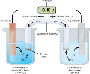
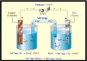
(II) Standard Cell Potentials (Voltaic Cells):

 Galvanic Cell

A galvanic cell is an important electrochemical cell. It is named after Luigi Galvani, an Italian physicist. It is also called a Voltaic cell, after an Italian physicist, Alessandro Volta. A galvanic cell generally consists of two different metal rods called electrodes. Each electrode is immersed in a solution containing its onions, and these form a half-cell. Each half-cell is connected by a salt bridge or separated by a porous membrane. The solutions in which the electrodes are immersed are called electrolytes.

The chemical reaction that takes place in a galvanic cell is the redox reaction. One electrode acts as the anode in which oxidation takes place, and the other acts as the cathode in which reduction takes place.  The best example of a galvanic cell is the Daniell cell.

The cell voltage is proportional to ΔG, the change in Gibbs free energy. The ΔG of the reaction could be harnessed to do useful electrical work. This thermodynamic equation gives the value of ΔG.

ΔG = ΔG° + RT ln Q  — (1)

The relationship between cell voltage, E, and ΔG for the cell reaction is given by the following equation.

DG = -nFE, or E = -DG/nF —(2), where n is number of electrons, F = 96485 J/mol.V

The Nernst equation showing the cell potential can be finally written as

 

        (or)     

Where E° = E°_1/2(reduction) − E°_1/2(oxidation)

E° = E°_1/2(cathode) − E°_1/2(anode)

In this investigation, you will make the following voltaic cells by using the following simulation:

http://amrita.olabs.edu.in/?sub=73&brch=8&sim=153&cnt=4

Activity series: Use cell notation and perform the virtual lab.

Part I		Part II
Anode             (oxidation)	Cathode       (reduction)	Anode            (oxidation)	Cathode       (reduction)
(1)   Mg/Mg2+(0.05 M) || Zn2+ (0.1 M)/Zn  (2)   Mg/Mg2+( (0.05 M) || 2Ag+ (0.1 M)/2Ag       (3)   Mg/Mg2+( (0.05 M) || Cu2+(0.1 M)/Cu (4)   Mg/Mg2+( (0.05 M) || Fe2+(0.1 M)/Fe (5)   Mg/Mg2+(0.05 M) || Ba2+ (0.1 M)/Ba		(6)   Zn/Zn2+(0.05 M) || Ba2+ (0.1 M)/Ba           (7)   Zn/Zn2+(0.05 M) || Mg2+ (0.1 M)/Mg             (8)   Zn/Zn2+ (0.05 M) || 2Ag+ (0.1 M)/2Ag  (9)   Zn/Zn2+ (0.05 M) || Cu2+(0.1 M)/Cu           (10)   Zn/Zn2+ (0.05 M) || Fe2+(0.1 M)/Fe

           

 Procedure:

You will create a series of voltaic cell models in two different parts: (i) Mg involves oxidation consistently, and other ions involve reduction, and (ii) Zn involves oxidation consistently, and other ions involve reduction.

Set the concentration of solution in the anode part (left) as 0.05 M, whereas the concentration of the solution in the cathode part is 0.1 M.

This setup is consistent for all 10 cell models where you can see the type of solutions (e.g., aqueous BaCl₂, MgCl₂, AgNO₃, ZnSO₄, CuSO₄ and FeSO₄) where cations are ionized in the solution.   

Part I:

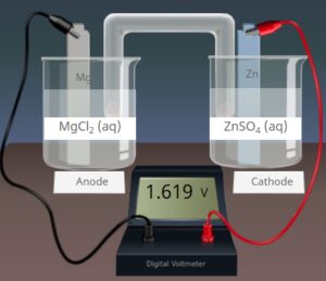
• Select the electrode Mg in the anode part (top), where MgCl₂ (the corresponding ionic solution) will appear in the beaker by default.
• Select the electrode Zn in the cathode part (bottom), where ZnSO₄ (the corresponding ionic solution) will appear in the beaker by default. This is model #1.
• Observe the cell potential (E_cell) from the digital voltmeter.
• Repeat the same procedure with the anode (Mg) and various cathodes (Ag, Cu, Fe and Ba) to complete the rest of the models (Models 2-5).

Part II:

• Select the electrode Zn in the anode part (top), where ZnSO₄ (the corresponding ionic solution) will appear in the beaker by default.
• Select the electrode Ba in the cathode part (bottom), where BaCl₂ (the corresponding ionic solution) will appear in the beaker by default. This is model #6…
• Observe the cell potential (E_cell) from the digital voltmeter.
• Repeat the same procedure with the anode (Zn) and various cathodes (Ag, Cu, Fe and Ba) to complete the rest of the models (Models 7-10).

Table: Cell potential measured for various voltaic cells (by using simulation) in comparison with the theoretical values.                     (10 points)                                                               

Voltaic cell	Electrodes	Anode	Cathode	Ecell, V (Exp.)	Ecell, V (Pred.)a	% Error
1	Mg & Zn	Mg/Mg2+(0.05 M)	Zn2+ (0.1 M)/Zn	1.619	1.619	0
2	Mg & Ag	Mg/Mg2+( (0.05 M)	2Ag+ (0.1M)/2Ag	3.17	3.25	-2.52
3	Mg & Cu	Mg/Mg2+( (0.05 M)	Cu2+(0.1 M)/Cu	2.71	2.79	-2.95
4	Mg & Fe	Mg/Mg2+( (0.05 M)	Fe2+(0.1 M)/Fe	1.93	2.01	-4.14
5	Mg & Ba	Mg/Mg2+(0.05 M)	Ba2+ (0.1 M)/Ba	-0.53	-0.44	-2.00
6	Zn & Ba	Zn/Zn2+(0.05 M)	Ba2+ (0.1 M)/Ba	-2.14	-2.05	16.9
7	Zn & Mg	Zn/Zn2+(0.05 M)	Mg2+ (0.1 M)/Mg	-1.61	-1.52	5.59
8	Zn & Ag	Zn/Zn2+ (0.05 M)	2Ag+ (0.1 M)/2Ag	1.56	1.64	-5.12
9	Zn & Cu	Zn/Zn2+ (0.05 M)	Cu2+(0.1 M)/Cu	1.1	1.18	-7.27
10	Zn & Fe	Zn/Zn2+ (0.05 M)	Fe2+(0.1 M)/Fe	0.32	0.40	25.0

^a Finish the answering question (a) and enter values here.

(a) Calculate the predicted E_cell value for each cell by the Nernst Equation. (20 points)

where n = 2 and Q = [0.05]/[0.1] à both are consistent in all 10 models

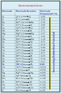
(1) Model calculation for Model #1: Collect the reduction potential from the table at the bottom of the PPT or other resources.

E^o = E^o(cathode) – E^o(anode) = (-0.76 V) – (-2.37 V) = +1.61 V

E = E^o – (0.0591/n) (log Q) = 1.61 – (0.0591/2) (log [0.05/0.1]) = 1.619 V

From the Desmos scientific calculator From the Virtual Lab:

 

The calculation for Model #2:

E^o = E^o(cathode) – E^o(anode) = (+0.80V) – (-2.37 V) = +3.17 V

E = E^o – (0.0591/n) (log Q) = 3.17 – (0.0591/2) (log [0.05/0.1]) = 3.25 V

Calculation for Model #3:

E^o = E^o(cathode) – E^o(anode) = (+0.34V) – (-2.37 V) = +2.71 V

 E = E^o – (0.0591/n) (log Q) = 2.71 – (0.0591/2) (log [0.05/0.1]) = 2.79 V

The calculation for Model #4:

E^o = E^o(cathode) – E^o(anode) = (-0.44V) – (-2.37 V) = +1.93 V

 E = E^o – (0.0591/n) (log Q) = 1.93 – (0.0591/2) (log [0.05/0.1]) = 2.01V

The calculation for Model #5:

E^o = E^o(cathode) – E^o(anode) = (-2.90V) – (-2.37 V) = -0.53 V

E = E^o – (0.0591/n) (log Q) = -0.53 – (0.0591/2) (log [0.05/0.1]) = -0.44V

Calculation for Model #6:

E^o = E^o(cathode) – E^o(anode) = (-2.90V) – (-0.76 V) = -2.14 V

 E = E^o – (0.0591/n) (log Q) = -2.14 – (0.0591/2) (log [0.05/0.1]) = -2.05 V

 Calculation for Model #7:

E^o = E^o(cathode) – E^o(anode) = (-2.37V) – (-0.76 V) = -1.61 V

 E = E^o – (0.0591/n) (log Q) = -1.61 – (0.0591/2) (log [0.05/0.1]) = -1.52 V

Calculation for Model #8:

E^o = E^o(cathode) – E^o(anode) = (+0.80V) – (-0.76 V) = +1.56 V

E = E^o – (0.0591/n) (log Q) = 1.56 – (0.0591/2) (log [0.05/0.1]) = 1.64V

Calculation for Model #9:

E^o = E^o(cathode) – E^o(anode) = (+0.34V) – (-0.76 V) = +1.1 V

E = E^o – (0.0591/n) (log Q) = 1.1 – (0.0591/2) (log [0.05/0.1]) = 1.18V

Calculation for Model #10:

E^o = E^o(cathode) – E^o(anode) = (-0.44V) – (-0.76 V) = +0.32 V

 E = E^o – (0.0591/n) (log Q) = 0.32 – (0.0591/2) (log [0.05/0.1]) = 0.40V

(b) Write an overall redox reaction for each voltaic cell first and then half-reactions, which are labeled “oxidation” and “reduction.”      (10 points)

Model 1: Mg/Mg2+ || Zn2+/Zn   Redox: Mg(s) + Zn2+(aq) à Mg2+(aq) + Zn(s)   Oxidation: Mg à Mg 2+ + 2e– Reduction: Zn2+ + 2e–  àZn	Model 6:     Zn/Zn2+ || Ba2+/Ba   Oxidation: Zn à Zn 2+ + 2e–   Reduction: Ba2+ + 2e–  àBa
Model 2:     Mg/Mg2+ || 2Ag+/ 2Ag   Oxidation: Mg à Mg 2+ + 2e–   Reduction: 2Ag2+ + 2e–  à2Ag	Model 7:   Zn/Zn2+ || Mg2+/Mg   Oxidation: Zn à Zn 2+ + 2e–   Reduction: Mg2+ + 2e–  àMg
Model 3:   Mg/Mg2+ || Cu2+/Cu     Oxidation: Mg à Mg 2+ + 2e–   Reduction: Cu2+ + 2e–  àCu	Model 8: Zn/Zn2+ || 2Ag+/2Ag   Oxidation: Zn à Zn 2+ + 2e–   Reduction: 2Ag2+ + 2e–  à2Ag
Model 4: Mg/Mg2+ || Fe2+/Fe   Oxidation: Mg à Mg 2+ + 2e–   Reduction: Fe2+ + 2e–  àFe	Model 9: Zn/Zn2+ || Cu2+/Cu   Oxidation: Zn à Zn 2+ + 2e–   Reduction: Cu2+ + 2e–  àCu
Model 5: Mg/Mg2+ || Ba2+/Ba   Oxidation: Mg à Mg 2+ + 2e–   Reduction: Ba2+ + 2e–  àBa	Model 10: Zn/Zn2+ || Fe2+/Fe   Oxidation: Zn à Zn 2+ + 2e–   Reduction: Fe2+ + 2e–  àFe

 

(c) Write a summary of the argument based on this simulation lab. (10 points)

From the simulations, it is evident that the standard electrode potentials provided determine whether a reaction will take place or not.  Also, the most reactive metals from the table undergo oxidation, thus strong reducing agents. The least reactive metals undergo reduction, hence strong oxidizing agents. The value of the electrode potential determines the position of a metal in a reactivity series. For example, copper has an electrode potential of +0.34 V, while magnesium has -2.37V. Therefore, copper cannot displace magnesium from a solution of its ions, but magnesium can displace copper. Overall, negative electrode potential from a complete cell indicates that a reaction cannot take place and vice versa.

 Appendix Table: Reduction potential for various electrode and reduction reactions.

ORDER A PLAGIARISM-FREE PAPER HERE

We’ll write everything from scratch

---

This is a lab practical; please complete all pages and show calculations and graphs as asked.