Course Project Worksheet – Calculating Sample Sizes Using G* Power
Variables: (Identify the variables used.)
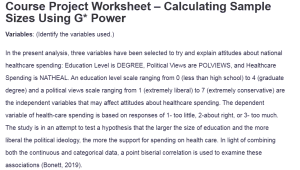
In the present analysis, three variables have been selected to try and explain attitudes about national healthcare spending: Education Level is DEGREE, Political Views are POLVIEWS, and Healthcare Spending is NATHEAL. An education level scale ranging from 0 (less than high school) to 4 (graduate degree) and a political views scale ranging from 1 (extremely liberal) to 7 (extremely conservative) are the independent variables that may affect attitudes about healthcare spending. The dependent variable of health-care spending is based on responses of 1- too little, 2-about right, or 3- too much. The study is in an attempt to test a hypothesis that the larger the size of education and the more liberal the political ideology, the more the support for spending on health care. In light of combining both the continuous and categorical data, a point biserial correlation is used to examine these associations (Bonett, 2019).
Test Family and Statistical Test: (Identify the test family and statistical test used.)
For this analysis, the t-test family was selected in G*Power and indicated that the statistical test is a correlation: point biserial model. The point biserial correlation is appropriate with these data since it examines the relationship between a continuous and a binary variable, an approach commonly utilized in social science research when one of the variables has only two categories. A two-tailed test allows observation of the association in either direction, so it is more balanced when we have no strong hypothesis about the direction of the effect.
G*Power Output:
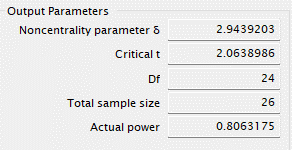
The G*Power output provided the following results:
- Noncentrality parameter δ: 2.9439
- Critical t: 2.0639
- Degrees of freedom (Df): 24
- Total sample size: 26
- Actual power: 0.8063
Output Parameters: (Explain each of the output parameters.)
The output parameters of G*Power are really useful in interpreting the reliability of the study and finding the sample size.
Noncentrality parameter (δ): This is the expected deviation from the null hypothesis given the specified effect size and sample size. The larger the noncentrality parameter, the easier it is under the chosen conditions; an effect of the relationship or difference being sought will be detected. In this case, the value of 2.9439 suggests that to some moderate departure, corresponding to a large effect size as selected.
Critical t: On this matter, the critical t, which is 2.0639, stands as the threshold beyond which the statistical significance will have transcended in this test. More to that, for a correlation to be regarded as statistically significant, the actual t-value obtained from the real data must exceed this critical value threshold. It sets a high threshold, and hence, the rejection of the null hypothesis at this threshold minimizes Type I errors.
Degrees of freedom: The degrees of freedom for the t-test is 24, as the sample size in total derived was 26. The degrees of freedom define the number of independent pieces of information used to calculate the estimate of the population parameters and from this definition, n−2 in the case of a correlation test. A greater degree of freedom will provide more precise estimates of statistical significance.
Overall sample size: To realize these power and effect size, a sample size of 26 participants shall be required. In other words, to realize 80% power in detecting an effect size of 0.5 (large) with a probability or significance of 0.05, we need at least 26 participants for this study. This is a crucial finding because it informs the researcher about the minimum sample size needed to achieve a balance between statistical power and practical feasibility (Aberson, 2019).
Actual power: The actual power yielded is 0.8063, which is slightly over the threshold of 0.80. This means that a probability of 80.63% exists for rejecting a false null hypothesis, which in turn minimizes the chances of occurrence of Type II error. In general, reaching a power level as close to 0.80 is acceptable in psychological and social sciences (Lakens, 2013) when a good balance is reached between reducing the risk of Type II errors and keeping the sample size feasible.
References
Aberson, C. L. (2019). Applied power analysis for the behavioral sciences. Routledge.
Bonett, D. G. (2019). Point‐biserial correlation: Interval estimation, hypothesis testing, meta‐analysis, and sample size determination. British Journal of Mathematical and Statistical Psychology. https://doi.org/10.1111/bmsp.12189
Lakens, D. (2013). Calculating and reporting effect sizes to facilitate cumulative science: A practical primer for t-tests and anovas. Frontiers in Psychology, 4(863). https://doi.org/10.3389/fpsyg.2013.00863
ORDER A PLAGIARISM-FREE PAPER HERE
We’ll write everything from scratch
Question 
Using the G* power website, download the free software and conduct a G* power analysis using the provided data.
There are 4 types of power analysis (a priori, post-hoc, criterion, and sensitivity). For the purposes of this class, we will focus on a priori power analysis since it is most commonly used when designing a research study (Hunt, n.d.).
Using the following parameters, complete a G* power analysis:
Alpha= .05
Power= .80
Expected Effect Size = In Week 2 Discussion 2, we practiced using the “Which Stats Test” Sage Tool.
Refer to the statistical test determined using that tool and select the large effect size for the appropriate test. (Note: if you aren’t sure which test to use, you can use the t-test family, correlation). You will not lose points for choosing the incorrect test. The point here is to determine a test, input the parameters into G*power, and explain the results.
Figure 1 – Effect Size Benchmarks
| Statistic | Small | Medium | Large |
| Means – Cohen’s d | 0.2 | 0.5 | 0.8 |
| ANOVA – f | 0.1 | 0.25 | 0.4 |
| ANOVA – eta squared | 0.01 | 0.06 | 0.14 |
| Regression f-test | 0.02 | 0.15 | 0.35 |
| Correlation – r or point serial | 0.1 | 0.3 | 0.5 |
| Correlation – r squared | 0.01 | 0.06 | 0.14 |
| Association – 2 x 2 table – OR | 1.5 | 3.5 | 9 |
| Association – Chi-square – w or Phi | 0.1 | 0.3 | 0.5 |
Source: Hunt. (n.d.). A researcher’s guide to power analysis. Utah State University. Retrieved from https://research.usu.edu/irb/wp-content/uploads/sites/12/2015/08/A_Researchers_Guide_to_Power_Analysis_USU.pdf
Course Project Worksheet – Calculating Sample Sizes Using G* Power
G* Power Analysis
Variables: (Identify the variables used.)
[Enter your response here.]
Test Family and Statistical Test: (Identify the test family and statistical test used.)
[Enter your response here.]
G*Power Output:
[Copy and paste your G*Power output here.]
Output Parameters: (Explain each of the output parameters.)
[Enter your response here.]
References
[List references according to APA guidelines.]