Discussion – Tests of Significance
Dependent Variable – Income.
Code – Conrinc
GSS measurement – Interval/ ratio –
Independent Variable – Education
Code – Educ
GSS measurement – Ordinal
Control Variable – Race
Code – RACE
GSS measurement – Ordinal
Hypothesis
Research Hypothesis; H1: There is a significant relationship between the dependent and independent variable
Null Hypothesis; H0: There is no significant relationship between the dependent and independent variable
ANOVA Analysis with DV and IV Variable
| ANOVA | |||||
| Respondent income in constant dollars | |||||
| Sum of Squares | df | Mean Square | F | Sig. | |
| Between Groups | 272067822400.000 | 19 | 14319359070.000 | 11.935 | .000 |
| Within Groups | 1610043590000.000 | 1342 | 1199734418.000 | ||
| Total | 1882111412000.000 | 1361 | |||
The p-value obtained at a .05 level of significance is .000 (p<.0001). This implies that we reject the null hypothesis and conclude that the relationship between the dependent and independent variables is significant.
Univariate Test with IV, DV, and Control Variable
| Univariate Tests | |||||
| Dependent Variable: Respondent income in constant dollars | |||||
| Sum of Squares | df | Mean Square | F | Sig. | |
| Contrast | 252334572100.000 | 19 | 13280766960.000 | 11.159 | .000 |
| Error | 1595956856000.000 | 1341 | 1190124427.000 | ||
| The F tests the effect of the Highest year of school completed. This test is based on the linearly independent pairwise comparisons among the estimated marginal means. | |||||
There p-value when using the independent variable, dependent variable, and control variable is also smaller than the alpha level, indicating there is a relationship between the dependent, independent, and control variables. This suggests further studies can be conducted for the variables.
ORDER A PLAGIARISM-FREE PAPER HERE
We’ll write everything from scratch
Question
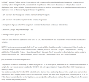
In Week 3, we used Epsilons and the 10-percent-point rule to determine if a potential relationship between two variables is worth examining further. During Weeks 4-5, we studied tests of significance. In this week’s discussion, we will apply these tests of significance to our project variables. As we discussed previously, the levels of measurement of our variables determine which test of significance works for the research project. Here are the guidelines:

Discussion – Tests of Significance
1. DV and IV are BOTH categorical variables (nominal/ordinal): Chi-square
2. DV and IV are both continuous (interval/ratio) variables: Regression
3. Comparison of groups (when IV is categorical – nominal/ordinal and DV is continuous – interval/ratio):
a. Between 2 groups: Independent Sample T-test
b. Among 3 or more groups: ANOVA
***Be sure to run the test of significance twice – once on ONLY the IV and the DV and once with the DV and both the IV and control variables.
NOTE: If running a regression analysis, both the IV and control variables should be moved to the independent(s) box. If running an ANOVA, the analysis with the control variable requires a different procedure. For IV/DV – Analyze – Compare Means – One Way ANOVA. For IV/Control/DV – Analyze – General Linear Model – Univariate. The IV is moved to the fixed factor box, and the control is moved to the covariate box. Click on EM Means, move IV over, click Compare Main Effects, and Choose Bonferroni.
Why do we need to run tests of significance?
They allow us to see if our relationship is “statistically significant.” To be more specific, these tests tell us if a relationship observed in a sample, like your research project based on the GSS 2018 data set, is generalizable to the population from which this sample was drawn (US adults).
Test results reported under “p” in the SPSS output tell us the chances that a relationship observed in the sample is not real but rather due to factors like a sampling error or chance. We compare this “chance” with alpha (level of significance), commonly set as .05 or .01. If this chance is smaller than the level of significance, we can reject the null hypothesis and keep the research hypothesis. The smaller the p, the lower the possibility for error.

