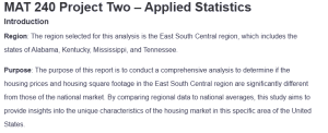
MAT 240 Project Two – Applied Statistics
Introduction
Region: The region selected for this analysis is the East South Central region, which includes the states of Alabama, Kentucky, Mississippi, and Tennessee.
Purpose: The purpose of this report is to conduct a comprehensive analysis to determine if the housing prices and housing square footage in the East South Central region are significantly different from those of the national market. By comparing regional data to national averages, this study aims to provide insights into the unique characteristics of the housing market in this specific area of the United States.
Sample: To have a representative and unbiased analysis, 500 valid house sales from the East South Central region were taken at random. This sample contains data for all four states in the region, along with specific details on each house listing, including state, county, house price, cost per square foot, and total square footage, among other things. In this study we examine a wide range of properties throughout the region in order to accurately capture the overall trends and patterns in the local housing market.
Questions and type of test: This analysis will focus on two primary research questions, each with its own hypothesis and corresponding statistical test
First hypothesis:
– Population parameter: The population parameter for the first hypothesis is the mean house listing price for homes in the East South Central region.
– Hypothesis: The hypothesis states that the mean housing price in the East South Central region is equal to or greater than $288,407, which is the mean of the national market. In other words, this hypothesis proposes that housing prices in the region are not significantly lower than the national average.
– Test: To evaluate this hypothesis, a 1-tailed test will be utilized. This type of test is appropriate when the alternative hypothesis specifies a directional difference (i.e., greater than or less than) between the sample mean and the hypothesized population mean.
Second hypothesis:
Population parameter: The population parameter for the second hypothesis is the mean square footage of houses in the East South Central region.
Hypothesis: The hypothesis proposes that the mean square footage of houses in the East South Central region is equal to or not equal to 1944 square feet, which represents the mean square footage of houses in the national market. This hypothesis aims to determine if there is a significant difference between the average house size in the region compared to the nation as a whole.
Test: A 2-tailed test will be used to assess this hypothesis. The 2-tailed test is suitable when the alternative hypothesis does not specify a directional difference but simply states that the sample mean differs from the hypothesized population mean.
Level of confidence: To further support the analysis and provide a range of plausible values for the true population mean, estimation and confidence intervals will be utilized. Specifically, a 95% confidence interval will be constructed to estimate the range of values within which the actual mean square footage of homes in the East South Central region is likely to fall. This level of confidence provides a balance between precision and reliability, allowing for reasonable certainty in the conclusions drawn from the data.
1-Tail Test
Hypothesis: The population parameter of interest for the first hypothesis is the mean house listing price for homes in the East South Central region. This parameter represents the average price at which houses are initially listed for sale in the region.
Hypothesis: Null (H0): The mean house listing price in the East South Central region is less than or equal to the national mean of $288,407.
-Alternative (Ha): The mean house listing price in the East South Central region is greater than the national mean of $288,407.
Hypothesis: The significance level, denoted as α, is set at 0.05 for this analysis
Data analysis:
Data analysis:
| House Listing Price Summary Statistics | |
| Mean | 228496.47 |
| Standard Error | 3996.86945 |
| Median | 211475 |
| Mode | 169950 |
| Standard Deviation | 89372.7179 |
| Sample Variance | 7987482700 |
| Range | 530950 |
| Minimum | 119000 |
| Maximum | 649950 |
Data analysis:
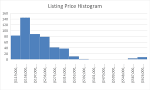
The summary statistics show that the sample mean price of $228,496 is far less than the national mean of $288,407. Chances are, on average, the houses in the East South Central region are listed at a lower price than the national average. The sample median of $211,475 is also about one-third lower than the national median of $249,940, and thus, the central tendency of housing prices in the region is lower than in the nation as a whole. The standard deviation of the data spread into house listing prices for the sample 89,372 is less than the national standard deviation of 172,779 when thinking about how quickly the data spreads. This means there is less variability in housing prices with East South Central region than the national market. The shape of the distribution is revealed in the histogram of the sample data. This is a right skewed histogram with an extended tail to higher prices. The skewness in this implies that for the most part, houses are spread out across the lower price range, but there are a few higher priced outliers that pull the mean up.
Data analysis: Before proceeding with the hypothesis test, we need to verify that the required conditions & assumptions are met. The sampling distribution of the sample mean appears to be normal in this case, which is the normal condition. The central limit theorem says that the distribution of sample means converges to normal if the sample size is large, regardless of the form of the original population. Assuming that the normal condition holds when the sample size is 500 is reasonable.
Hypothesis Test Calculations: The standard error was computed by dividing the sample standard deviation by the square root of the sample size.
Standard error = $89,372 / sqrt(500) = $3,996.87
The test statistic was then calculated using the following formula:
t = (sample mean – hypothesized population mean) / standard error
t = ($228,496 – $228,407) / $3,996.87 = -14.99
Hypothesis Test Calculations: Using the T.DIST function in Excel, the p-value was determined as 5.23 x 10E.107
Interpretation: To interpret the results of the hypothesis test, we compare the p-value to the predetermined significance level (α) of 0.05. In this case, the p-value of 1.67029E-42 is far below the significance level. When the p-value is less than α, we reject the null hypothesis in favor of the alternative hypothesis.
Interpretation: Based on the low p-value of 1.67029E-42, which is less than the significance level of 0.05, we reject the null hypothesis
Interpretation: Rejecting the null hypothesis allows us to conclude that there is sufficient evidence to support the claim that the mean house listing price in the East South Central region is lower than the national mean of $288,407. This finding suggests that housing prices in the region are significantly more affordable compared to the national average.
2-Tail Test
Hypotheses: The population parameter of interest for the second hypothesis is the mean square footage of houses in the East South Central region. This parameter represents the average size of homes in the region, measured in square feet.
Hypotheses: Null (H0): The mean square footage of houses in the East South Central region is equal to the national mean of 1944 square feet.
Alternative (Ha): The mean square footage of houses in the East South Central region is not equal to the national mean of 1944 square
Hypotheses: The significance level (α) is set at 0.05
Data Analysis:
Data Analysis:
| Square Footage Summary Statistics | |
| Mean | 2030.84643 |
| Standard Error | 16.5084985 |
| Median | 1988 |
| Mode | 2000 |
| Standard Deviation | 369.141248 |
| Sample Variance | 136265.261 |
| Kurtosis | 3.51485417 |
| Skewness | 0.69793506 |
| Range | 3109.64286 |
| Minimum | 342.857143 |
| Maximum | 3452.5 |
| Sum | 1015423.21 |
| Count | 500 |
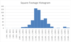
Data Analysis: Although the sample mean square footage is slightly higher than the national mean (2,031 vs. 1944), the houses appear smaller in the East South Central region than the national average. Specifically, however, the difference is much less pronounced than in house listing prices. Interestingly, the sample median square footage of 1,988 is more than the national median of 1,881. This in fact means that the regional mean value for house sizes is actually less than the national median house size. The square footage standard deviation in the sample is slightly lower (369.14) than the national one (385). This implies that house sizes are not more variable in the East South Central region than in the national market. The sample data histogram shows a very slightly skewed to the right distribution with a very long tail towards higher square footage. The mean implies that most of these houses are grouped around the central value, but there are other houses that cast a larger shadow in terms of the mean.
Data Analysis: According to the central limit theorem, the large size of the sample of 500 ensures that the normal condition is generally met. Regardless of the shape of the population distribution, if we are lucky enough to have a sufficiently large sample, then the sampling distribution of the sample mean tends to be normal. The independence assumption is likely to hold because the data was obtained using a random sampling method. With random sampling, you know that each house has an equal chance of being selected and that the selection of one house does not depend on the selection of another. Furthermore, no apparent violations exist for the conditions needed for hypothesis testing.
Hypothesis Test Calculations: t = (2,031 – 1944) / 16.51 = 5.26
Hypothesis Test Calculations: The T.DIST.2T function in Excel was used and the resulting p-value was 1.57465E-06.
Interpretation: To interpret the results, we compare the p-value to the significance level (α) of 0.05. In this case, the p-value of 1.57465E-06 is well below the significance level. When the p-value is less than α, we reject the null hypothesis in favor of the alternative hypothesis.
Interpretation: Based on the p-value of 1.57465E-06, which is below the significance level of 0.05, we reject the null hypothesis.
Interpretation: Since we have rejected the null hypothesis, we can conclude that there is enough evidence to suggest that the mean square footage of houses in the East South Central region is significantly different from the national mean of 1944 square feet. This finding means the average house size in the region is statistically distinct from the national
Comparison of the Test Results: To provide a range of plausible values for the true mean square footage in the region, a 95% confidence interval was constructed.
Margin of error = 1.96 x 16.51 = 32.43
The confidence interval is:
– Lower bound: 2,031 – 32.43 = 1,998.57
– Upper bound: 2,031 + 32.43 = 2,063.43
Thus, we can be 95% confident that the true mean square footage of homes in the region lies between 1,998.57 and 2,063.43 square feet.
Final Conclusions
Summarize Your Findings: Significant differences between the East South Central housing market and the national housing market are revealed in terms of housing prices. Homes in this region are significantly better priced than the rest of the nation, evidenced by the sample’s mean listing price of $228,496, which is quite substantially less than the national mean of $288,407. This difference is significant at a 95% confidence level, and the hypothesis test confirms this. As for square footage, the mean house size in the area is 2,031 square feet, slightly above the national average of 1944 square feet. Since the size difference is small, it is statistically highly significant, implying that homes in the area are, on average, a bit smaller. Second, we estimate the 95% confidence interval, which is the true mean square footage for the region according to the range from 1,998.57 to 2,063.43 square feet.
Discuss: The findings of this analysis were both expected and unexpected. As expected, housing prices in the East South Central region are significantly lower than the national average with the southeastern U.S. generally being less expensive to live in. In particular, the magnitude of the difference was apparent, with the national mean price being nearly $59,910 less than the regional mean. This stark contrast indicates the region’s affordability of homes, thus notably highlighting that home buyers in the region may likely have far greater purchasing power than the other parts of the country in exercise of the buying limits.
However, when it came to the results in square feet, some were unexpected. While the mean square footage was less than the national average, the disparity was not as great as first envisioned. The median square footage of the sample was higher than the national median, which is interesting, considering that while the average home size is slightly smaller, there are a huge number of large homes in the region. The statistically significant difference in square footage portrays, while the size gap is not as dramatic as the price gap, an important distinction about the East South Central housing market. But statistically, homes in the region aren’t particularly small – the 95% confidence interval for square footage indicates a reasonable amount of living space for homes, even if they’re a little smaller on average than the national norm.
ORDER A PLAGIARISM-FREE PAPER HERE
We’ll write everything from scratch
Question 
Competency
In this project, you will demonstrate your mastery of the following competency:
- Apply statistical techniques to address research problems
- Perform hypothesis testing to address an authentic problem
Overview
In this project, you will apply inference methods for means to test your hypotheses about the housing sales market for a region of the United States. You will use appropriate sampling and statistical methods.
Scenario
You have been hired by your regional real estate company to determine if your region’s housing prices and housing square footage are significantly different from those of the national market. The regional sales director has three questions that they want to see addressed in the report:
- Are housing prices in your regional market lower than the national market average?
- Is the square footage for homes in your region different than the average square footage for homes in the national market?
- For your region, what is the range of values for the 95% confidence interval of square footage for homes in your market?
You are given a real estate data set that has houses listed for every county in the United States. In addition, you have been given national statistics and graphs that show the national averages for housing prices and square footage. Your job is to analyze the data, complete the statistical analyses, and provide a report to the regional sales director. You will do so by completing the Project Two Template located in the What to Submit area below.
Directions
Introduction
- Region: Start by picking one region from the following list of regions:
West South Central, West North Central, East South Central, East North Central, Mid Atlantic - Purpose: What is the purpose of your analysis?
- Sample: Define your sample. Take a random sample of 500 house sales for your region.
- Describe what is included in your sample (i.e., states, region, years or months).
- Questions and type of test: For your selected sample, define two hypothesis questions (see the Scenario above) and the appropriate type of test for each. Address the following for each hypothesis:
- Describe the population parameter for the variable you are analyzing.
- Describe your hypothesis in your own words.
- Identify the hypothesis test you will use (1-Tail or 2-Tail).
- Level of confidence: Discuss how you will use estimation and confidence intervals to help you solve the problem.
1-Tail Test
- Hypothesis: Define your hypothesis.
- Define the population parameter.
- Write null (Ho) and alternative (Ha) hypotheses. Note: For means, define a hypothesis that is less than the population parameter.
- Specify your significance level.
- Data analysis: Summarize your sample data using appropriate graphical displays and summary statistics and confirm assumptions have not been violated to complete this hypothesis test.
- Provide at least one histogram of your sample data.
- In a table, provide summary statistics including sample size, mean, median, and standard deviation. Note: For quartiles 1 and 3, use the quartile function in Excel:
=QUARTILE([data range], [quartile number]) - Summarize your sample data, describing the center, spread, and shape in comparison to the national information (under Supporting Materials, see the National Summary Statistics and Graphs House Listing Price by Region PDF). Note: For shape, think about the distribution: skewed or symmetric.
- Check the conditions.
- Determine if the normal condition has been met.
- Determine if there are any other conditions that you should check and whether they have been met. Note: Think about the central limit theorem and sampling methods.
- Hypothesis test calculations: Complete hypothesis test calculations.
- Calculate the hypothesis statistics.
- Determine the appropriate test statistic (t). Note: This calculation is (mean – target)/standard error. In this case, the mean is your regional mean, and the target is the national mean.
- Calculate the probability (p value). Note: This calculation is done with the T.DIST function in Excel:
=T.DIST([test statistic], [degree of freedom], True) The degree of freedom is calculated by subtracting 1 from your sample size.
- Calculate the hypothesis statistics.
- Interpretation: Interpret your hypothesis test results using the p value method to reject or not reject the null hypothesis.
- Relate the p value and significance level.
- Make the correct decision (reject or fail to reject).
- Provide a conclusion in the context of your hypothesis.
MAT 240 Project Two – Applied Statistics
2-Tail Test
- Hypotheses: Define your hypothesis.
- Define the population parameter.
- Write null and alternative hypotheses. Note: For means, define a hypothesis that is not equal to the population parameter.
- State your significance level.
- Data analysis: Summarize your sample data using appropriate graphical displays and summary statistics and confirm assumptions have not been violated to complete this hypothesis test.
- Provide at least one histogram of your sample data.
- In a table, provide summary statistics including sample size, mean, median, and standard deviation. Note:For quartiles 1 and 3, use the quartile function in Excel:
=QUARTILE([data range], [quartile number]) - Summarize your sample data, describing the center, spread, and shape in comparison to the national information. Note:For shape, think about the distribution: skewed or symmetric.
- Check the assumptions.
-
-
- Determine if the normal condition has been met.
- Determine if there are any other conditions that should be checked on and whether they have been met. Note: Think about the central limit theorem and sampling methods.
-
- Hypothesis test calculations: Complete hypothesis test calculations.
- Calculate the hypothesis statistics.
-
-
- Determine the appropriate test statistic (t). Note: This calculation is (mean – target)/standard error. In this case, the mean is your regional mean, and the target is the national mean.]
- Determine the probability (p value). Note: This calculation is done with the TDIST.2T function in Excel:
=T.DIST.2T([test statistic], [degree of freedom]) The degree of freedom is calculated by subtracting 1 from your sample size.
-
- Interpretation: Interpret your hypothesis test results using the p value method to reject or not reject the null hypothesis.
- Compare the pvalue and significance level.
- Make the correct decision (reject or fail to reject).
- Provide a conclusion in the context of your hypothesis.
- Comparison of the test results: Revisit Question 3 from the Scenario section: For your region, what is the range of values for the 95% confidence interval of square footage for homes?
- Calculate and report the 95% confidence interval. Show or describe your method of calculation.
Final Conclusions
- Summarize your findings: In one paragraph, summarize your findings in clear and concise plain language.
- Discuss: Discuss whether you were surprised by the findings. Why or why not?