MAT 240 Project One Guidelines

Introduction

This report aims to develop a predictive model based on the square footage of housing prices. D. M. Pan National Real Estate Company, therefore, instructed me to come up with a model that will help real estate agents estimate the listing prices using square footage as a benchmark. With the novelty of housing data from 2019, this paper will attempt to demystify the following central research question: Is the square footage a good predictor in ascertaining housing prices? Companies dealing in real estate, like D.M. Pan, rely on predictive models so that the listing prices are as accurate as possible. In that way, they can develop better pricing strategies and be able to provide better recommendations to their clients. While the relationship between the size of a home and its price is well documented, determining how significant this factor in isolation can be, agents may find value. Linear regression is the chief analytical tool used in this report. Linear regression would be appropriate for this context; it looks at the relationship between two variables, one of which predicts the other.

The developed model will attempt to determine if a linear relationship does exist between square footage predictor variable- and listing the response variable. This would imply that for linear regression to apply, there must be a linear trend in the underlying relationship between the response and predictor variable. Here, it is expected that the scatterplot will show an upward trend with higher square footage, and the listing price will rise. In that case, it would mean that based on linearity, the scatterplot with a trend line would indicate that square footage can predict listing prices. A nonlinear relationship could suggest the use of more complex models.

Any linear regression model just defines a predictor and a response variable. For this model, square footage would be the predictor variable since the hypothesis is on the independent variable driving the dependent variable, listing price. The house price corresponds to a response variable. What is important to know is how much of the variation in listing prices can be explained by changes in square footage and how reliable this relationship is to carry forward for making future predictions.

Data Collection

I randomly sampled 50 houses from all the regions to start the analysis. Using all regions is quite fitting, as it provides a diverse sample of house sizes and prices. Random sampling ensures that all observations have an equal chance of being included in the analysis, which helps reduce sampling bias. In this case, the sample was generated using Excel’s random number generator. This was accomplished by adding a new column to the spreadsheet and naming it “random,” then typing in the formula `=RAND()` to create random numbers for each listing. Sorting these random numbers along with the rest of the data allowed me to select the first 50 entries for the analysis. This avoided human bias that might have occurred had I handpicked houses, based perhaps on visual appeal or other presumptions about value.

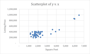
Figure 1: Scatterplot of y v. x

Data Analysis

Histogram of Square Feet

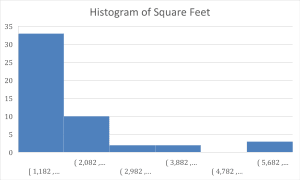
Figure 2: Square Feet Histogram

Histogram of Listing Price

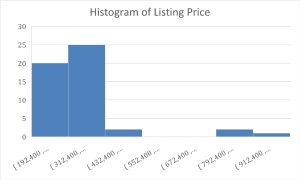
Figure 3: Listing Price Histogram

Summary statistics

	Listing Price	Square Feet
Mean	359,472	2,254
Median	340,550	1,862
Std. Dev.	155282.631	1171.889586

Table 1: Summary Statistics

From Figure 2, it’s observable that the histogram of square footage suggests most homes in the sample fall between 1,182 and 2,082 square feet. That is to say, most of the samples are smaller homes. The distribution is right-skewed, meaning there are fewer homes with larger square footage, but the values for those larger homes are much higher. This is not out of the ordinary in real estate data since only a few homes tend to be abnormally larger than the median size.

Figure 3 shows the same picture in detail from the histogram of listing prices: most homes fall within the prices of $192,400 to $432,400. It is also right-skewed since there aren’t too many houses in that range of price. The above data reflects what generally happens out in the housing market: homes become fewer yet much more costly.

Summary statistics describe central tendencies and dispersion. Below, Table 1 provides a table of important summary statistics for both listing price and square footage. There are several key conclusions from the table: First, we can see the mean listing price was $359,472, which is above the national average of $342,365. This suggests that the houses in our sample are generally more expensive than the typical house on the national level. On the other hand, however, the median listing price is lower than the mean value at $340,550, indicating a few high-priced homes in the sample, thereby pulling the mean upwards. At an average square footage of 2,254 square feet, these are barely above the national average of 2,111 square feet. This would, therefore, mean that most homes in the sample of the Pacific region were larger than the national average.

The median listing price, $340,550, is still a little lower than the mean listing price. This is indicative that there are few high-priced outliers driving up the mean. This is not unusual in housing data since high-end luxury homes often drive up averages. In square footage, the median is 1,862 square feet and is lower than the mean, indicating there may be larger homes, which drive up the mean square footage.

Spread: The large standard deviation for the listing price ($155,282) and square footage (1,171) indicates significant dispersion in the data. As we could anticipate with a sample of this size, several homes are much larger and far more expensive than others. A variation of this type will go a long way toward ensuring that the regression model will be robust and applicable to a great variety of homes.

Shape: Because most of the houses are clustered in a lower range both for square footage and listing price, there is a right-skewed distribution for both variables. In the case of normal housing data, that’s usually how it works: more homes exist within a mid-range price bracket than in higher brackets that reach into luxury.

We could compare sample statistics to national statistics as a way to determine if the sample appears to be representative of the nation’s housing market. The sample mean listing price is $359,472; this number is slightly higher than the national average listing price of $342,365. Correspondingly, the sample median listing price is $340,550, somewhat higher than the national median listing price of $318,000. By square footage, the sample mean involves 2,254 square feet, which is slightly larger than the national mean of 2,111 square feet. Similarly, the sample median of 1,862 square feet is close to the national median of 1,881 square feet. With some slight differences, these statistics would support that the sample is reasonably representative of the nation, although it may be slightly biased toward larger homes and higher listing prices.

Develop Regression Model

Scatterplot

This scatterplot displays a positive linear relationship where square footage is the predictor variable listing price is the response variable. As the values of square footage increase, listing prices also tend to increase. The overall relationship is approximately linear in that the points generally follow a straight-line pattern, but there is a bit of variability. This is a fairly strong association, as can be seen by the tight clustering of points along the trendline-and it says that square footage is a key predictor of the listing price.

In this scatterplot, one could imagine there are a few outliers, especially at the high ends of square footage and listing price. These points are much further away from the crowd of data and may target making a difference in correlation. Generally speaking, outliers represent special cases, like costly luxury estates or homes in prime places, and may thus turn the results a bit by exaggerating the relationship between feet and price.

Without the outliers, the model would likely have a weaker relationship between square footage and listing price. It is important not to remove these outliers from the analysis because they represent real data that reflects higher-end homes. In this respect, allowing them to remain in the model incorporates variability for a wider range of properties, hence making it more robust and useful for listing price predictions of a greater variety of homes.

The correlation coefficient was approximately 0.871, which says there is a great positive linear relationship between the square footage and listing price. The scatterplot’s line of best fit is often aligned with the high value of r Hover for the points. This implies that the listing price may be accurately predicted by square footage.

Determine the Line of Best Fit

The regression equation, which is also the line of best fit, is as follows:

y = 115.42x + 99276

In this equation, the slope ( 115.42) represents the rate at which the listing price increases for each additional square foot. The intercept (99276) is the estimated listing price for a home with zero square feet, which may not have practical significance but is necessary for the regression model.

The slope of 115.42 indicates that for every additional square foot of a house, the listing price increases by approximately $115.42. This suggests that larger homes tend to be listed at higher prices, reflecting the real estate industry’s general space valuation. The intercept, 99,276, suggests that even a house with very little square footage would still have a base price due to factors like land value, neighborhood, or amenities.

The R-squared value for the regression equation is approximately 0.76, meaning that 76% of the variability in listing price can be explained by the square footage of the home. This indicates that the model has strong predictive power, though 24% of the variability remains unexplained by square footage alone. Other factors like location, property condition, and market trends likely influence the listing price.

Using the regression equation y = 115.42x + 99,276, we can predict the listing price for a home with 1,500 square feet of living space. Using the equation we can have:

y = 115.42(1500) + 99,276

= 173,130 + 99,276

= 272,406

Thus, for a 1,500-square-foot home, the predicted listing price would be approximately $272,406. This prediction assumes that the only factor influencing price is square footage, which, while important, may overlook other significant contributors like location or property condition.

Conclusions

In sum, this analysis has demonstrated that square footage is a robust predictor of listed price in properties. The positive linear trend in the data, reflected by the correlation coefficient of 0.871, indicates that an increase in square footage leads to a corresponding increase in the list price of the property. Our regression model explains 76% of the variation in listing prices, indicating that, for these homes, square footage is a major determinant of home value. Real estate agents could use such information to better estimate prices when setting listing prices with respect to home size.

The findings were pretty much as expected since bigger houses usually have a higher market price. On the other hand, the incidence of a few outliers was not exactly anticipated, especially for huge square footage houses. In this case, those outliers most likely correspond to luxury properties or houses in highly desired locations.

Adding further variables, such as location, age of the home, or amenities nearby, would enhance the model, allow for nuance within the predictions, and could explain the variability that may be unaccounted for with the current model. Another potential improvement would be segregation between regions or types of homes in attempts to more fully capture the diversity within the housing market. How do market trends, including interest rates and economic conditions, influence listing prices in real estate over time?. This could provide valuable insights into how external factors influence home values in different regions.

ORDER A PLAGIARISM-FREE PAPER HERE

We’ll write everything from scratch

---

Competencies

In this project, you will demonstrate your mastery of the following competencies:

• Apply statistical techniques to address research problems
• Perform regression analysis to address an authentic problem

Overview

The purpose of this project is to have you complete all of the steps of a real-world linear regression research project starting with developing a research question, then completing a comprehensive statistical analysis, and ending with summarizing your research conclusions.

Scenario

You have been hired by the D. M. Pan National Real Estate Company to develop a model to predict housing prices for homes sold in 2019. The CEO of D. M. Pan wants to use this information to help their real estate agents better determine the use of square footage as a benchmark for listing prices on homes. Your task is to provide a report predicting the housing prices based square footage. To complete this task, use the provided real estate data set for all U.S. home sales as well as national descriptive statistics and graphs provided.

Directions

Using the Project One Template located in the What to Submit section, generate a report including your tables and graphs to determine if the square footage of a house is a good indicator for what the listing price should be. Reference the National Statistics and Graphs document for national comparisons and the Real Estate Data Spreadsheet spreadsheet (both found in the Supporting Materials section) for your statistical analysis.

Note: Present your data in a clearly labeled table and using clearly labeled graphs.

Specifically, include the following in your report:

Introduction

1. Describe the report: Give a brief description of the purpose of your report.
   1. Define the question your report is trying to answer.
   2. Explain when using linear regression is most appropriate.
      1. When using linear regression, what would you expect the scatterplot to look like?
   3. Explain the difference between predictor (x) and response (y) variables in a linear regression to justify the selection of variables.

Data Collection

1. Sampling the data: Select a random sample of 50 houses. Describe how you obtained your sample data (provide Excel formulas as appropriate).
   1. Identify your predictor and response variables.
2. Scatterplot: Create a scatterplot of your predictor and response variables to ensure they are appropriate for developing a linear model.

Data Analysis

1. Histogram: Create a histogram for each of the two variables.
2. Summary statistics: For your two variables, create a table to show the mean, median, and standard deviation.
3. Interpret the graphs and statistics:
   1. Based on your graphs and sample statistics, interpret the center, spread, shape, and any unusual characteristic (outliers, gaps, etc.) for house sales and square footage.
   2. Compare and contrast the center, shape, spread, and any unusual characteristic for your sample of house sales with the national population (under Supporting Materials, see the National Summary Statistics and Graphs House Listing Price by Region PDF). Determine whether your sample is representative of national housing market sales.

Develop Your Regression Model

1. Scatterplot: Provide a scatterplot of the variables with a line of best fit and regression equation.
   1. Based on your scatterplot, explain if a regression model is appropriate.
2. Discuss associations: Based on the scatterplot, discuss the association (direction, strength, form) in the context of your model.
   1. Identify any possible outliers or influential points and discuss their effect on the correlation.
   2. Discuss keeping or removing outlier data points and what impact your decision would have on your model.
3. Calculate r: Calculate the correlation coefficient (r).
   1. Explain how the r value you calculated supports what you noticed in your scatterplot.

Determine the Line of Best Fit. Clearly define your variables. Find and interpret the regression equation. Assess the strength of the model.

1. Regression equation: Write the regression equation (i.e., line of best fit) and clearly define your variables.
2. Interpret regression equation: Interpret the slope and intercept in context. For example, answer the questions: what does the slope represent in this situation? What does the intercept represent? Revisit the Scenario above.
3. Strength of the equation: Provide and interpret R-squared.
   1. Determine the strength of the linear regression equation you developed.
4. Use regression equation to make predictions: Use your regression equation to predict how much you should list your home for based on the assumed square footage of your home at 1500 square feet.

Conclusions

1. Summarize findings: In one paragraph, summarize your findings in clear and concise plain language for the CEO to understand. Summarize your results.
   1. Did you see the results you expected, or was anything different from your expectations or experiences?
   2. What changes could support different results, or help to solve a different problem?
   3. Provide at least one question that would be interesting for follow-up research.

You can use the following tutorial that is specifically about this assignment. Make sure to check the assignment prompt for specific numbers used for national statistics. The videos may use different national statistics. You should use the national statistics posted with this assignment.

• MAT-240 Module 4 Project One Video

What to Submit

To complete this project, you must submit the following:

Project One Template Word Document: Use this template to structure your report, and submit the finished version as a Word document. Submit your Excel file.

Supporting Materials

The following resources may help support your work on the project:

Document: National Summary Statistics and Graphs Real Estate Data PDF
Use this data for input in your project report.

Spreadsheet: Real Estate Data Spreadsheet
Use this data for input in your project report.

Tutorial: Downloading Office 365 Programs PDF
Use this tutorial for support with Office 365 programs.

Use these tutorials for support with the Excel functions you will use in the project: