Descriptive Statistics for Variables
Topic Question – Does an individual level of education determine their income?
Goal – To understand factors that affect/ determine income.
Dependent Variable – Income.
Code – Content
GSS Measurement – Interval
Question: What is your income in constant dollars?
Answer Categories: 0=IAP, 999998=DK, 999999=NA
Independent Variable – Education Level
Code – Educ
GSS Measurement – Ordinal
Question: What is your highest school year completed?
Answer Categories: 97=IAP, 98=DK, 99=NA.
Control Variable – Race
Code – RACE
GSS Measurement – Ordinal
Question: What is your race?
Answer Categories: 0=IAP, 1=YES, 2=NO, 8=DK, 9=NA.
Frequency Tables
“Inapplicable” (IAP), “Don’t know” (DK), and “No answer” (NA) are all considered to be invalid responses and are examples of “missing data” in SPSS; therefore, no inferences about them. The following analysis contains the valid entries.
Respondent income in constant dollars |
|||||
| Frequency | Percent | Valid Percent | Cumulative Percent | ||
| Valid | 351 | 33 | 1.4 | 2.4 | 2.4 |
| 1402 | 32 | 1.4 | 2.3 | 4.8 | |
| 2454 | 32 | 1.4 | 2.3 | 7.1 | |
| 3155 | 21 | .9 | 1.5 | 8.7 | |
| 3856 | 21 | .9 | 1.5 | 10.2 | |
| 4557 | 12 | .5 | .9 | 11.1 | |
| 5258 | 18 | .8 | 1.3 | 12.4 | |
| 6309 | 33 | 1.4 | 2.4 | 14.8 | |
| 7886 | 48 | 2.0 | 3.5 | 18.3 | |
| 9639 | 46 | 2.0 | 3.4 | 21.7 | |
| 11391 | 25 | 1.1 | 1.8 | 23.6 | |
| 13144 | 36 | 1.5 | 2.6 | 26.2 | |
| 14896 | 61 | 2.6 | 4.5 | 30.7 | |
| 16649 | 46 | 2.0 | 3.4 | 34.0 | |
| 19278 | 73 | 3.1 | 5.4 | 39.4 | |
| 22782 | 96 | 4.1 | 7.0 | 46.4 | |
| 26287 | 81 | 3.4 | 5.9 | 52.4 | |
| 31545 | 136 | 5.8 | 10.0 | 62.4 | |
| 38555 | 114 | 4.9 | 8.4 | 70.7 | |
| 47317 | 114 | 4.9 | 8.4 | 79.1 | |
| 57832 | 81 | 3.4 | 5.9 | 85.0 | |
| 70100 | 67 | 2.9 | 4.9 | 89.9 | |
| 84120 | 43 | 1.8 | 3.2 | 93.1 | |
| 98140 | 32 | 1.4 | 2.3 | 95.5 | |
| 112160 | 14 | .6 | 1.0 | 96.5 | |
| 182696 | 48 | 2.0 | 3.5 | 100.0 | |
| Total | 1363 | 58.0 | 100.0 | ||
| Missing | IAP | 985 | 42.0 | ||
| Total | 2348 | 100.0 | |||
The highest number of participants earn a constant income of 31545 dollars at 5.8%. The least number of respondents earn a constant income of 4557 dollars with 0.5%.
Highest year of school completed. |
|||||
| Frequency | Percent | Valid Percent | Cumulative Percent | ||
| Valid | 0 | 4 | .2 | .2 | .2 |
| 1 | 2 | .1 | .1 | .3 | |
| 2 | 4 | .2 | .2 | .4 | |
| 3 | 10 | .4 | .4 | .9 | |
| 4 | 5 | .2 | .2 | 1.1 | |
| 5 | 3 | .1 | .1 | 1.2 | |
| 6 | 20 | .9 | .9 | 2.0 | |
| 7 | 8 | .3 | .3 | 2.4 | |
| 8 | 35 | 1.5 | 1.5 | 3.9 | |
| 9 | 51 | 2.2 | 2.2 | 6.1 | |
| 10 | 65 | 2.8 | 2.8 | 8.8 | |
| 11 | 95 | 4.0 | 4.1 | 12.9 | |
| 12 | 657 | 28.0 | 28.0 | 40.9 | |
| 13 | 183 | 7.8 | 7.8 | 48.7 | |
| 14 | 313 | 13.3 | 13.3 | 62.0 | |
| 15 | 127 | 5.4 | 5.4 | 67.5 | |
| 16 | 430 | 18.3 | 18.3 | 85.8 | |
| 17 | 97 | 4.1 | 4.1 | 89.9 | |
| 18 | 119 | 5.1 | 5.1 | 95.0 | |
| 19 | 45 | 1.9 | 1.9 | 96.9 | |
| 20 | 72 | 3.1 | 3.1 | 100.0 | |
| Total | 2345 | 99.9 | 100.0 | ||
| Missing | DK | 2 | .1 | ||
| NA | 1 | .0 | |||
| Total | 3 | .1 | |||
| Total | 2348 | 100.0 | |||
The analysis of education levels indicates that the largest proportion of respondents (28%) have completed 12 years of education, which indicates that most respondents have only completed the basic primary and post-primary education. The second highest education years completed was 16, representing 12.8% of respondents, implying an undergraduate level of education.
Race of respondent |
|||||
| Frequency | Percent | Valid Percent | Cumulative Percent | ||
| Valid | WHITE | 1693 | 72.1 | 72.1 | 72.1 |
| BLACK | 385 | 16.4 | 16.4 | 88.5 | |
| OTHER | 270 | 11.5 | 11.5 | 100.0 | |
| Total | 2348 | 100.0 | 100.0 | ||
The whites contributed the larger proportion of respondents at 72.1%, followed by blacks at 16.4%, and other races constituted 11.5%. A large number of white respondents is due to the random selection of participants in the US.
| Descriptive Statistics | ||||
| Respondent income in constant dollars | Highest year of school completed | Race of respondent | ||
| N | Valid | 1363 | 2345 | 2348 |
| Missing | 985 | 3 | 0 | |
| Mean | 36812.71 | 13.73 | 1.39 | |
| Median | 26287.50 | 14.00 | 1.00 | |
| Mode | 31545 | 12 | 1 | |
| Std. Deviation | 37178.303 | 2.974 | .685 | |
| Variance | 1382226208.000 | 8.847 | .469 | |
The mean is a sufficient measure of central tendency in most cases since it uses all the data points and values in the data. However, since the data has a large number of missing values for each variable, the median is the best measure of central tendency. Also, since the data does not have extreme values that could make the mean biased, it is a sufficient measure of central tendency (Jones, 2015). The median for each variable shows where the responses were concentrated and shows the responses from the largest number of respondents. For instance, the median value of 1 for the races indicates that most of the respondents who responded were whites. As a measure of dispersion, the standard deviation is the best measure for all the variables since it contains all the characteristics that a data sample contains. The standard deviation is also not affected by the effects due to sampling, like other measures of dispersion. The standard deviation values indicate that the data has a small deviation from the mean.

Histograms
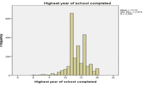
The highest average number of school years completed was 12 years, with a frequency of 657 respondents. The second-highest average number of school years completed was 16 years, with 430 respondents.

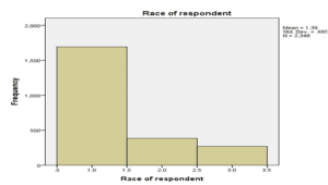
The mean frequency for the race of respondents indicate that the highest number of respondents were whites, since the mean tends to 1 (Whites category).

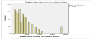
From the analysis, the highest number of respondents earned between $0-$50000 constant income. Thus, the data for the average income is skewed to the right.
References
Jones, P. (2015). When to use each measure of Central Tendency. Retrieved from https://courses.lumenlearning.com/introstats1/chapter/when-to-use-each-measure-of-central-tendency/
ORDER A PLAGIARISM-FREE PAPER HERE
We’ll write everything from scratch
Question 
Now that you have imported the GSS 2018 dataset into your SPSS and have learned how to use SPSS or the GSS data explorer to find out GSS variable information, you are going to create and post a frequency table, chart and descriptives table (central tendency/dispersion) of your variables. Complete the following steps:
Descriptive Statistics for Variables
Give your discussion a unique title specific to your study/variables. Post a brief explanation of your topic, which includes a bit of information about your variables: level of measurement, answer categories (yes/no, strongly agree, disagree, etc.), as well as the survey question used to collect data for this particular variable (refer to Discussion 1).
Include a frequency table for each of your variables. Explain your outputs for each variable in no more than 5 sentences. Cite numbers in the outputs to support your conclusion. When you cite %, use the % reported in the “valid percent” column.
Describe the measures of central tendency (mean, median, mode) and dispersion (variance, standard deviation) for each of your variables. Based on what you have learned in the readings and lessons this week, identify the best measures for each variable and explain what they tell us. What do these measures summarize for us about the variable’s data?
Presenting your data in graphic form is also important when conducting quantitative research. Based on what you have learned from the reading and the weekly lesson, create a graphic representation of your data. Your choice of graphing tool is purely based on a variable’s level of measurement. Explain your outputs for each variable. It is OK if your explanation is similar to (but not the same as) the frequency table interpretation since a chart is a different data presentation on the SAME variable. Cite numbers in the outputs to support your conclusion.
Copy all of the frequency tables and charts into the discussion window or into a document (PDF, MS Word) and attach to discussion. If your table/chart does not fit to the page, choose “copy special” and then “images” or take a screen shot of the table/chart. Paste images to a Word document.